Chapter 6 Advanced Usage

First, we build a CYT object with data in the extended data of CytoTree and build the tree-shaped trajectory.

# Loading packages
suppressMessages({
library(CytoTree)
})

# Read fcs files
fcs.path <- system.file("extdata", package = "CytoTree")
fcs.files <- list.files(fcs.path, pattern = '.FCS$', full = TRUE)

fcs.data <- runExprsMerge(fcs.files, comp = FALSE, transformMethod = "none")

# Refine colnames of fcs data
recol <- c(`FITC-A<CD43>` = "CD43", `APC-A<CD34>` = "CD34", 
           `BV421-A<CD90>` = "CD90", `BV510-A<CD45RA>` = "CD45RA", 
           `BV605-A<CD31>` = "CD31", `BV650-A<CD49f>` = "CD49f",
           `BV 735-A<CD73>` = "CD73", `BV786-A<CD45>` = "CD45", 
           `PE-A<FLK1>` = "FLK1", `PE-Cy7-A<CD38>` = "CD38")
colnames(fcs.data)[match(names(recol), colnames(fcs.data))] = recol
fcs.data <- fcs.data[, recol]

# Build the CYT object
cyt <- createCYT(raw.data = fcs.data, normalization.method = "log")

# Run CytoTree as pipeline and visualize as tree
set.seed(1)
cyt <- cyt %>% runCluster() %>% processingCluster() %>% 
  runFastPCA() %>% runTSNE() %>%  runDiffusionMap() %>% runUMAP() %>% 
  buildTree()
plotPieTree(cyt)

6.1 Fetch meta data

The first advanced usage is to fetch plot meta information of CytoTree.

# Fetch plot meta information for each cell
plot.meta <- fetchPlotMeta(cyt)
knitr::kable(head(plot.meta))

# Fetch plot meta information for each cluster
cluster.meta <- fetchClustMeta(cyt)
knitr::kable(head(cluster.meta))

6.2 Add meta data

The second advanced usage of CytoTree is to add meta-information to meta.data

# Old stage back up
plot.meta <- fetchPlotMeta(cyt)
old.stage <- plot.meta$stage

# Add meta-information in CytoTree meta.data
meta.information <- gsub(".FCS.+", "", rownames(fcs.data))
meta.information[!meta.information %in% "D0"] <- "not_D0"
names(meta.information) <- rownames(fcs.data)

# Change stage 
cyt <- addMetaData(cyt, meta.info = meta.information, name = "stage")
plotPieTree(cyt)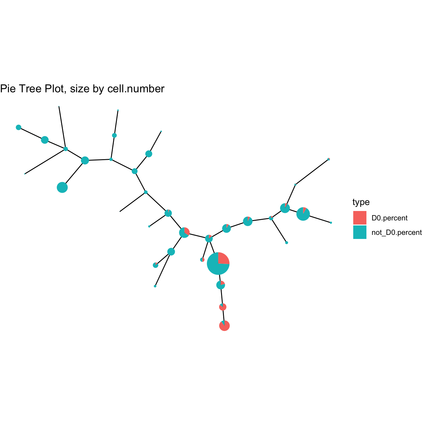

# Run PCA and view cell information as our new column
cyt <- runFastPCA(cyt)
cyt <- addMetaData(cyt, meta.info = meta.information, name = "Mycol")
plot2D(cyt, color.by = "Mycol", item.use = c("PC_1", "PC_2"))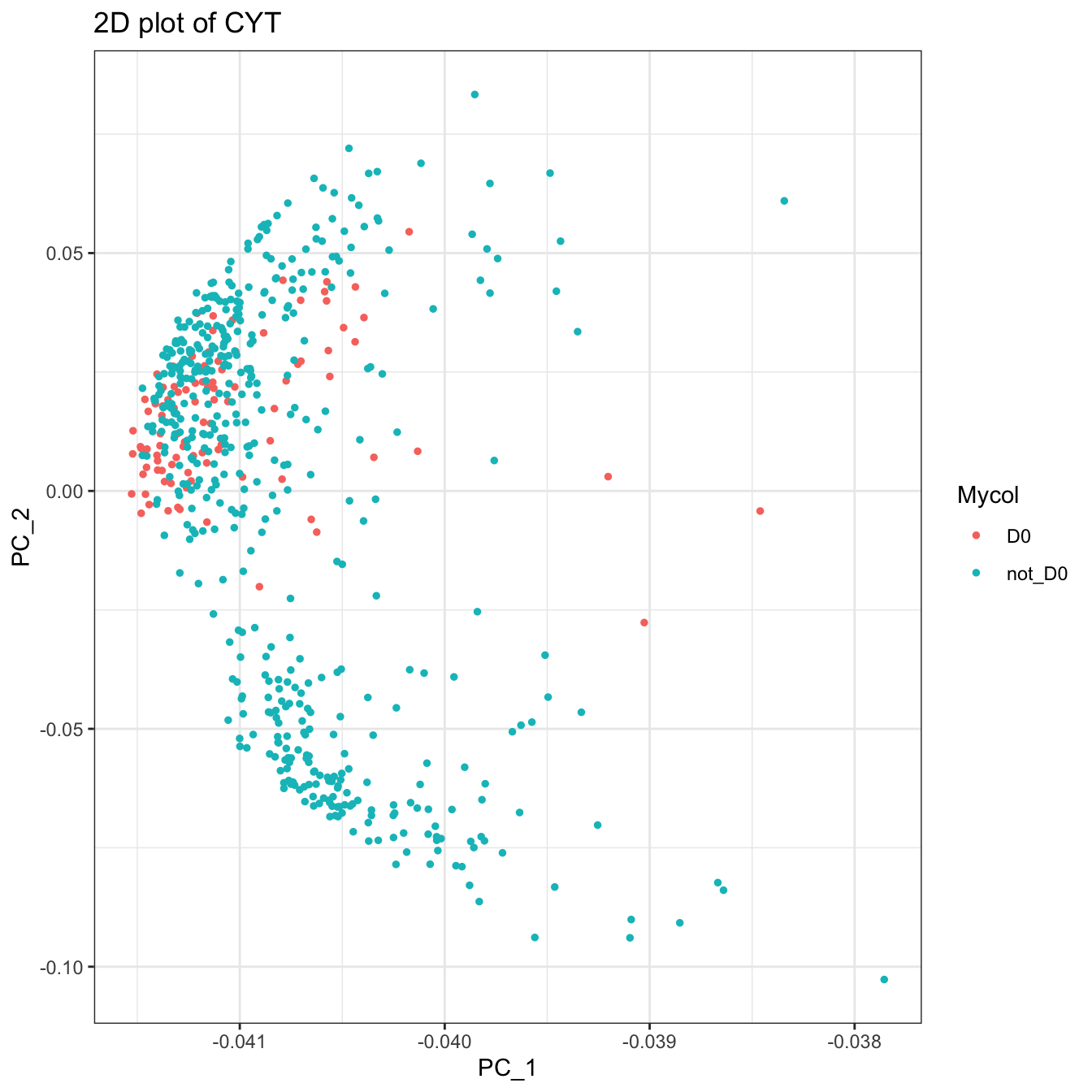

# Recover old stage 
cyt <- addMetaData(cyt, meta.info = old.stage, name = "stage")
plotPieTree(cyt)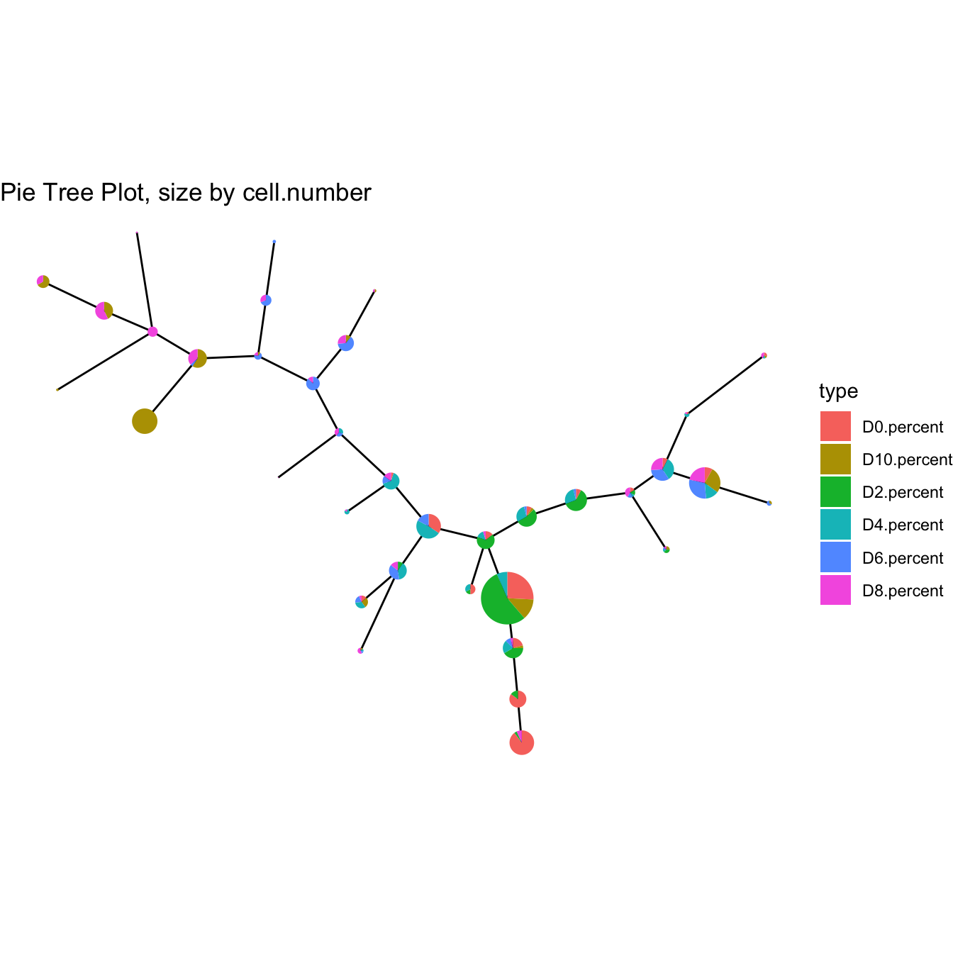

6.3 Fetch cells

Fetch cells using fetchCell

# Fetch cells 
cell.fetch <- fetchCell(cyt, stage = c("D0", "D10"))

6.4 Subset object

# Fetch cells 
cell.fetch <- fetchCell(cyt, stage = c("D0", "D10"))

# Subset object 
cyt.sub <- subsetCYT(cyt, cells = cell.fetch)
cyt.sub

## CYT Information:
##  Input cell number: 200  cells 
##  Enroll marker number: 10  markers 
##  Cells after downsampling: 200  cells

6.5 Batch effect

CytoTree provides function to correct batch effects based on ComBat in sva R package. Users can use `correctBatchCYT` to call it.

# Correct batch effect in building the CYT object
batch <- gsub(".FCS.+", "", rownames(fcs.data))
batch <- as.numeric(as.factor(batch))

# Build the CYT object without batch correction
cyt <- createCYT(raw.data = fcs.data, normalization.method = "log")

# Run CytoTree as pipeline and visualize as tree
set.seed(1)
cyt <- cyt %>% runCluster() %>% processingCluster() %>% 
  runFastPCA() %>% runTSNE() %>%  runDiffusionMap() %>% runUMAP() %>% 
  buildTree()
plot2D(cyt, item.use = c("UMAP_1", "UMAP_2"), color.by = "stage")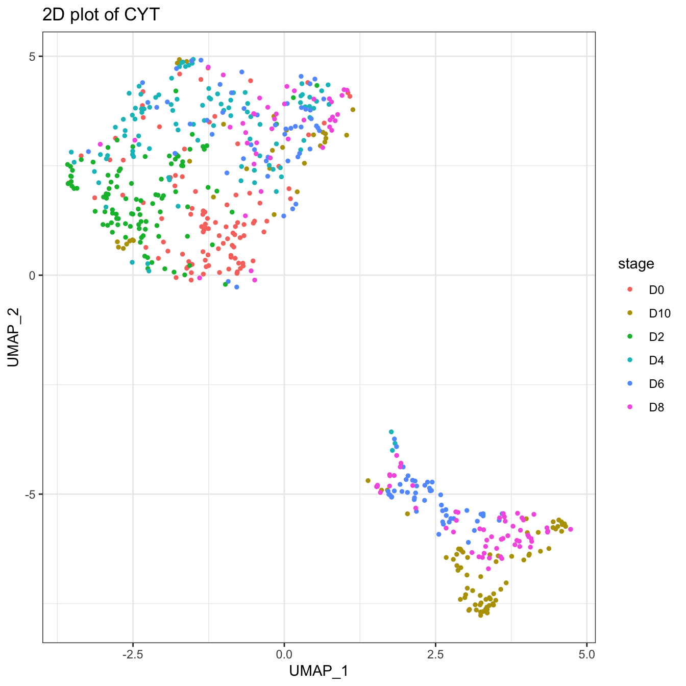

# Correct batch and re-run the pipeline
cyt <- correctBatchCYT(cyt, batch = batch)
set.seed(1)
cyt <- cyt %>% runCluster() %>% processingCluster() %>% 
  runFastPCA() %>% runTSNE() %>%  runDiffusionMap() %>% runUMAP() %>% 
  buildTree()
plot2D(cyt, item.use = c("UMAP_1", "UMAP_2"), color.by = "stage")

# Or build the CYT object with batch correction
cyt <- createCYT(raw.data = fcs.data, 
                 batch = batch, batch.correct = TRUE,
                 normalization.method = "log")

# Run CytoTree as pipeline and visualize as tree
set.seed(1)
cyt <- cyt %>% runCluster() %>% processingCluster() %>% 
  runFastPCA() %>% runTSNE() %>%  runDiffusionMap() %>% runUMAP() %>% 
  buildTree()
plot2D(cyt, item.use = c("UMAP_1", "UMAP_2"), color.by = "stage")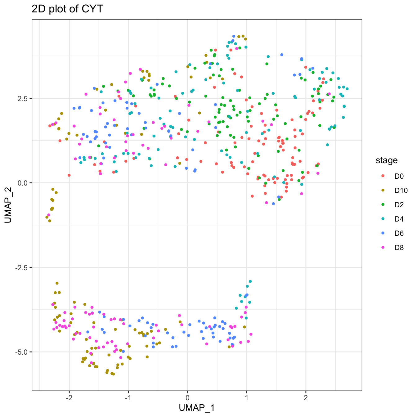

6.6 Change markers

The default option in CytoTee is to use all markers to calculate the tree-shaped trajectory. If we only want to use a subset of markers, for example, the CD Markers, we can use changeMarker to change markers in the calculation or change them in the building of the CYT object.

# Build the CYT object without batch correction
cyt <- createCYT(raw.data = fcs.data, normalization.method = "log")
set.seed(1)
cyt <- cyt %>% runCluster() %>% processingCluster() %>% 
  buildTree()
plotPieTree(cyt)

# Show all markers
knitr::kable(cyt@markers)

x
CD43
CD34
CD90
CD45RA
CD31
CD49f
CD73
CD45
FLK1
CD38

markers.cal <- c("CD43","CD34","CD90","CD45RA","CD49f","CD45","FLK1","CD38")


# Change markers using changeMarker
# This change will not change the raw.data in CTY object
cyt <- changeMarker(cyt, markers = markers.cal)
set.seed(1)
cyt <- cyt %>% runCluster() %>% processingCluster() %>% 
  buildTree()
plotPieTree(cyt)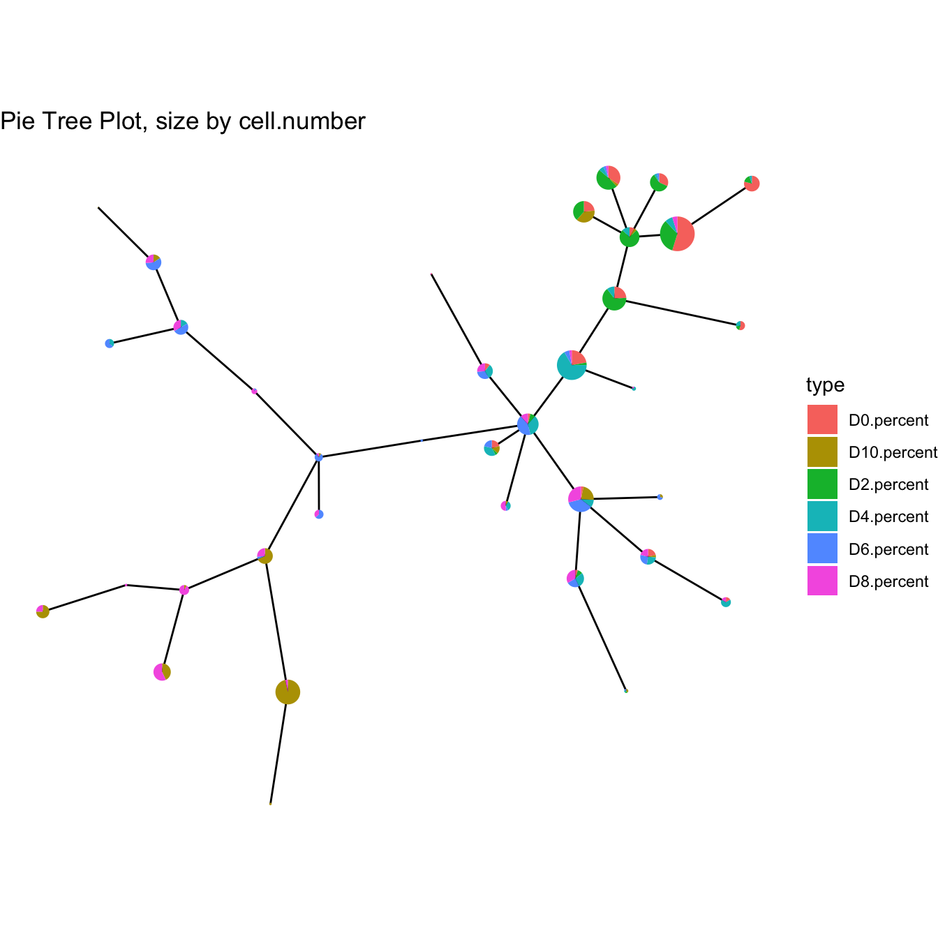

# Or change markers using createCYT
# This change will not change the raw.data in CTY object
cyt <- createCYT(raw.data = fcs.data, markers = markers.cal,
                 normalization.method = "log")
set.seed(1)
cyt <- cyt %>% runCluster() %>% processingCluster() %>% 
  buildTree()
plotPieTree(cyt)