Chapter 5 Time-course data use case

To illustrate the usage of CytoTree on differential trajectory reconstruction of time-course FCS data, we used a flow cytometry dataset of ten-day hematopoietic differentiation from the hESC line HUES9 on the basis of some modification of the previous work. By adding different cytokine combinations on different days, HUES9 cells (CD90+CD49f+ on Day 0, D0) were directionally differentiated into mesodermal cells (FLK1+, D4), hemogenic endothelium (CD34+CD31+CD43-, D6) and hematopoietic stem/progenitor cells (HSPCs, CD34+CD43+CD38-CD45RA-CD90+, D8) in succession. Ten cell surface markers (CD90, CD49f, FLK1, CD34, CD31, CD73, CD43, CD45, CD45RA, and CD38) were used for the flow cytometry analysis to monitor the generation of these cells.

This tutorial contains key steps of CytoTree time-course workflow, including how to calculate the pseudotime and how to define cell subsets and rebuild an CYT object using CytoTree. This use case also provided a framework for time-course cytometric data analysis and might provide support for research on stem cell reprogramming.

The data in this chapter can be download from GitHub via git clone https://github.com/JhuangLab/CytoTree-dataset.git.

And through this chapter, you will learn:

• 1. How to run time course cytometry data using CytoTree.
• 2. A framework for time course cytometry data analysis
• 3. How to illustrate the biological process using CytoTree.

5.1 Step 1. Preprocessing

# Loading packages
suppressMessages({
library(ggplot2)
library(pheatmap)
library(CytoTree)
library(stringr)
})

#########################
# Read Flow Cytometry Data
# It can be downloaded via `git clone https://github.com/ytdai/CytoTree-dataset.git` 
# fcs.path musted be modified based on the download directory from GitHub
fcs.path <- "FCS/time_course/"
fcs.files <- paste0(fcs.path, "D", c(0,2,4,6,8,10), ".fcs")

###########################################
#   Get the expression matrix from FCS file
###########################################

set.seed(1)
fcs.data <- runExprsMerge(fcs.files, comp = F, transformMethod = "none", fixedNum = 2000)

# Refine colnames of fcs data
# for usecase 2
recol <- c(`FITC-A<CD43>` = "CD43", `APC-A<CD34>` = "CD34", 
           `BV421-A<CD90>` = "CD90", `BV510-A<CD45RA>` = "CD45RA", 
           `BV605-A<CD31>` = "CD31", `BV650-A<CD49f>` = "CD49f",
           `BV 735-A<CD73>` = "CD73", `BV786-A<CD45>` = "CD45", 
           `PE-A<FLK1>` = "FLK1", `PE-Cy7-A<CD38>` = "CD38")
colnames(fcs.data)[match(names(recol), colnames(fcs.data))] = recol
fcs.data <- fcs.data[, recol]

# Build a CYT object
# If you don't want to see the running log information, set verbose FALSE
day.list <- c("D0", "D2", "D4", "D6", "D8", "D10")
meta.data <- data.frame(cell = rownames(fcs.data),
                        stage = str_replace(rownames(fcs.data), regex("_.+"), "") )
meta.data$stage <- factor(as.character(meta.data$stage), levels = day.list)

markers <- c("CD43", "CD34", "CD90", "CD45RA", "CD31", "CD49f", "CD73", "CD45", "FLK1", "CD38")

cyt <- createCYT(raw.data = fcs.data, markers = markers,
                 meta.data = meta.data,
                 normalization.method = "log")

5.2 Step 2. Trajectory

# Cluster cells by SOM algorithm
# Set random seed to make results reproducible
set.seed(80)
cyt <- runCluster(cyt, cluster.method = "som", xdim = 6, ydim = 6)

# Do not perform downsampling
set.seed(2)
cyt <- processingCluster(cyt, downsampling.size = 1)

# run Principal Component Analysis (PCA)
cyt <- runFastPCA(cyt)

# run t-Distributed Stochastic Neighbor Embedding (tSNE)
set.seed(1)
cyt <- runTSNE(cyt)

# run Diffusion map
cyt <- runDiffusionMap(cyt)

# run Uniform Manifold Approximation and Projection (UMAP)
cyt <- runUMAP(cyt)

# build minimum spanning tree based on UMAP
cyt <- buildTree(cyt, dim.type = "umap", dim.use = 1:2)

###########################################
# This is a visualization part
###########################################

# Plot marker density
plotMarkerDensity(cyt)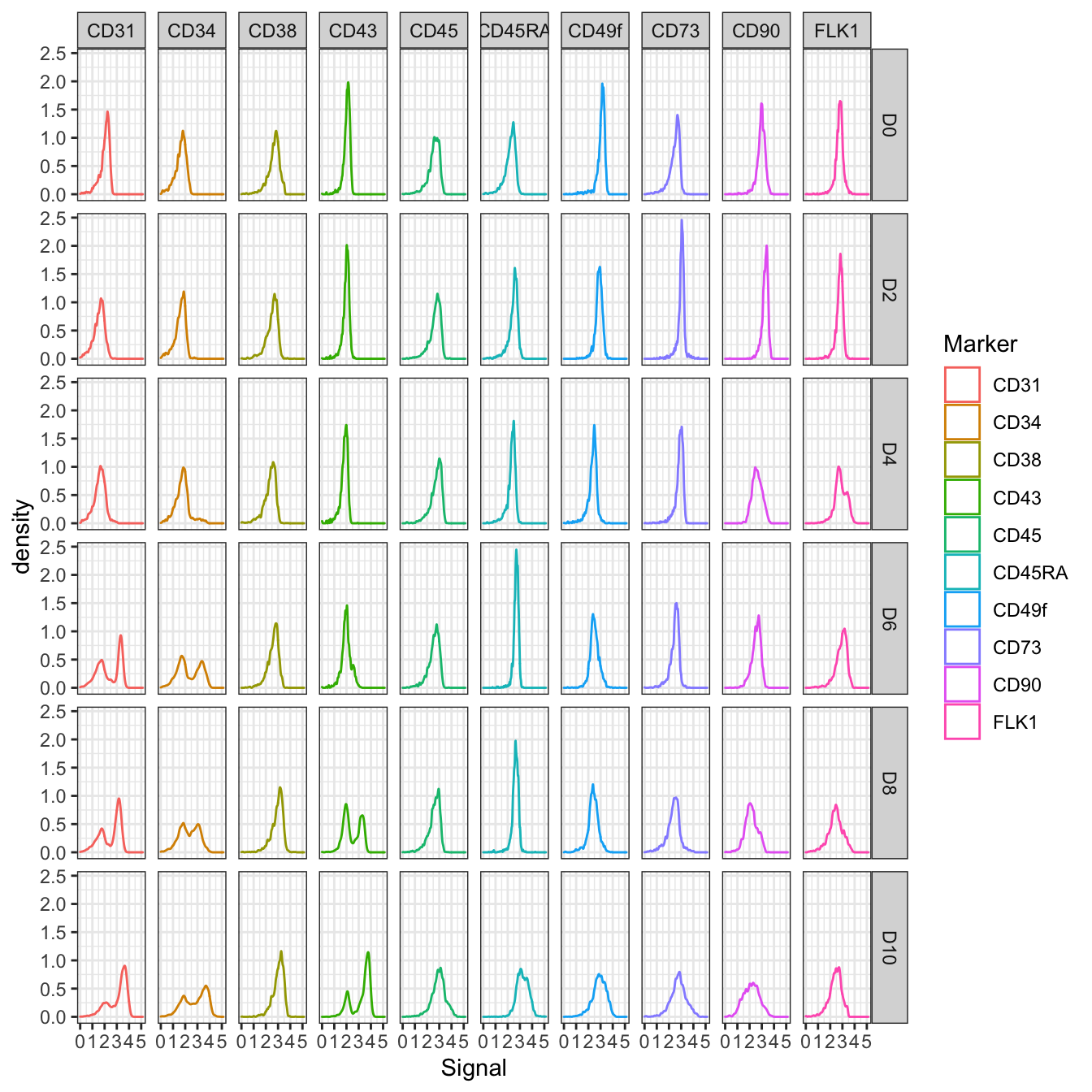

# Plot 2D PCA. And cells are colored by stage
plot2D(cyt, item.use = c("PC_1", "PC_2"), color.by = "stage", 
       alpha = 1, main = "tSNE", category = "categorical") + 
  scale_color_manual(values = c("#00599F","#009900","#FF9933",
                               "#FF99FF","#7A06A0","#FF3222"))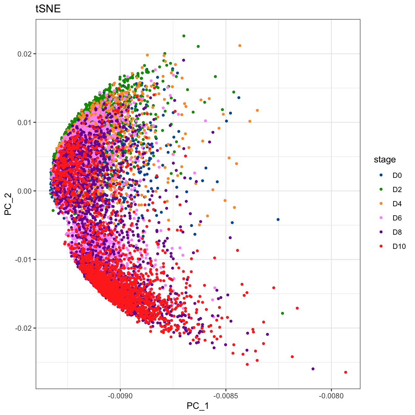

# Plot 2D tSNE. And cells are colored by stage
plot2D(cyt, item.use = c("tSNE_1", "tSNE_2"), color.by = "stage", 
       alpha = 1, main = "tSNE", category = "categorical") + 
  scale_color_manual(values = c("#00599F","#009900","#FF9933",
                               "#FF99FF","#7A06A0","#FF3222"))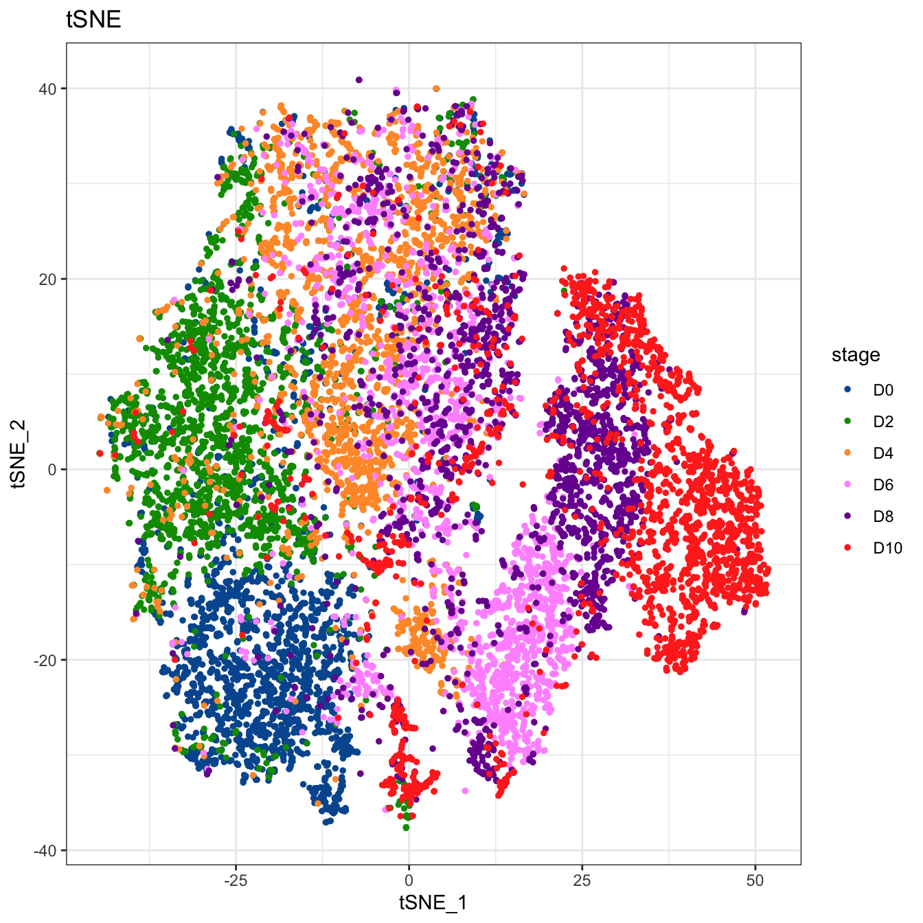

# Plot 2D diffusion maps. And cells are colored by stage
plot2D(cyt, item.use = c("DC_1", "DC_2"), color.by = "stage", 
       alpha = 1, main = "tSNE", category = "categorical") + 
  scale_color_manual(values = c("#00599F","#009900","#FF9933",
                               "#FF99FF","#7A06A0","#FF3222"))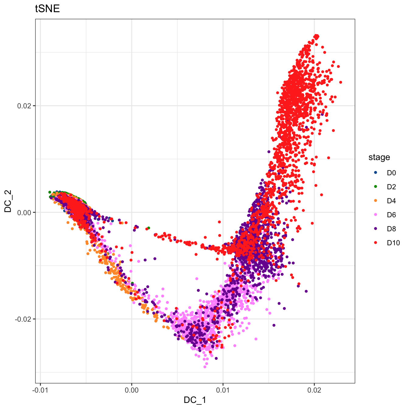

# Plot 2D UMAP. And cells are colored by stage
plot2D(cyt, item.use = c("UMAP_1", "UMAP_2"), color.by = "stage", 
       alpha = 1, main = "tSNE", category = "categorical") + 
  scale_color_manual(values = c("#00599F","#009900","#FF9933",
                               "#FF99FF","#7A06A0","#FF3222"))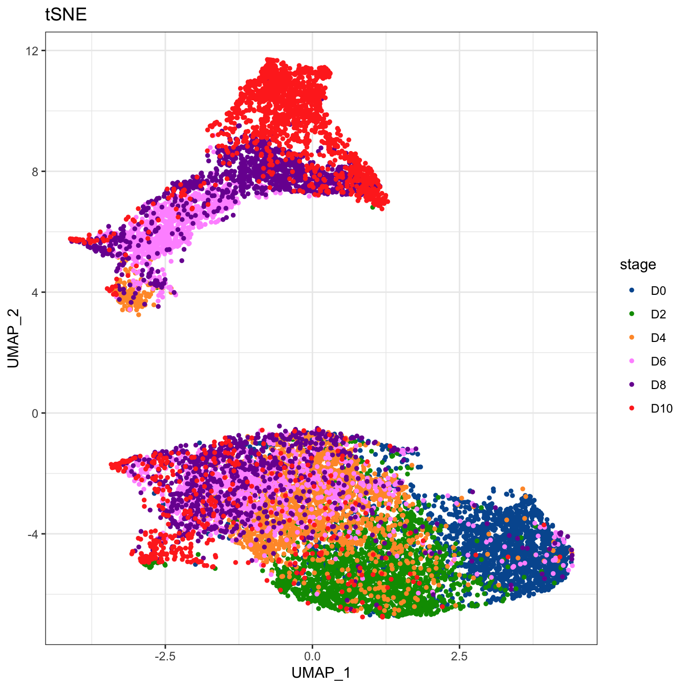

# Plot 2D tSNE. And cells are colored by cluster id
plot2D(cyt, item.use = c("tSNE_1", "tSNE_2"), color.by = "cluster.id", 
       alpha = 1, main = "tSNE", category = "categorical", show.cluser.id = T)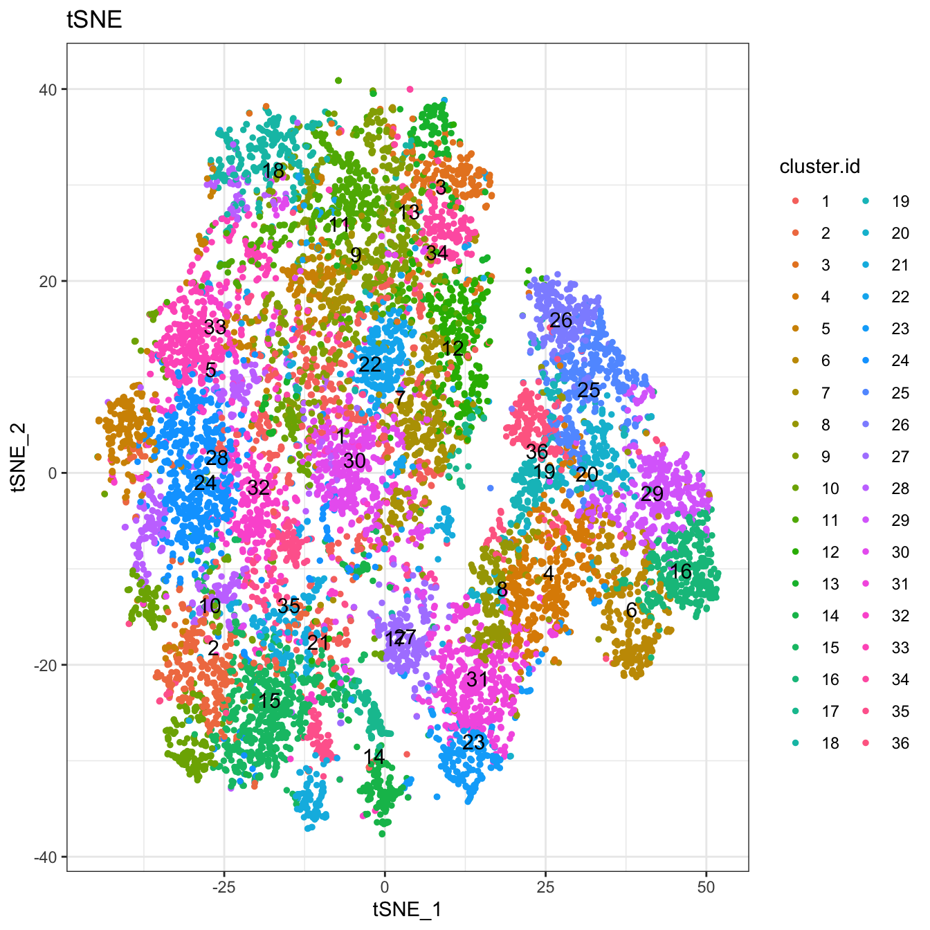

# Plot 2D UMAP. And cells are colored by cluster id
plot2D(cyt, item.use = c("UMAP_1", "UMAP_2"), color.by = "cluster.id", 
       alpha = 1, main = "UMAP", category = "categorical", show.cluser.id = T)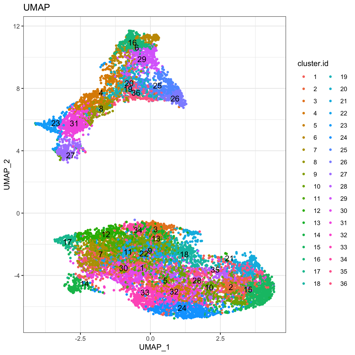

# Plot 2D tSNE. And cells are colored by CD43 markers expression
plot2D(cyt, item.use = c("tSNE_1", "tSNE_2"), color.by = "CD43", 
               main = "tSNE CD43", category = "numeric")  + 
 scale_colour_gradientn(colors = c("#00599F","#EEEEEE","#FF3222"))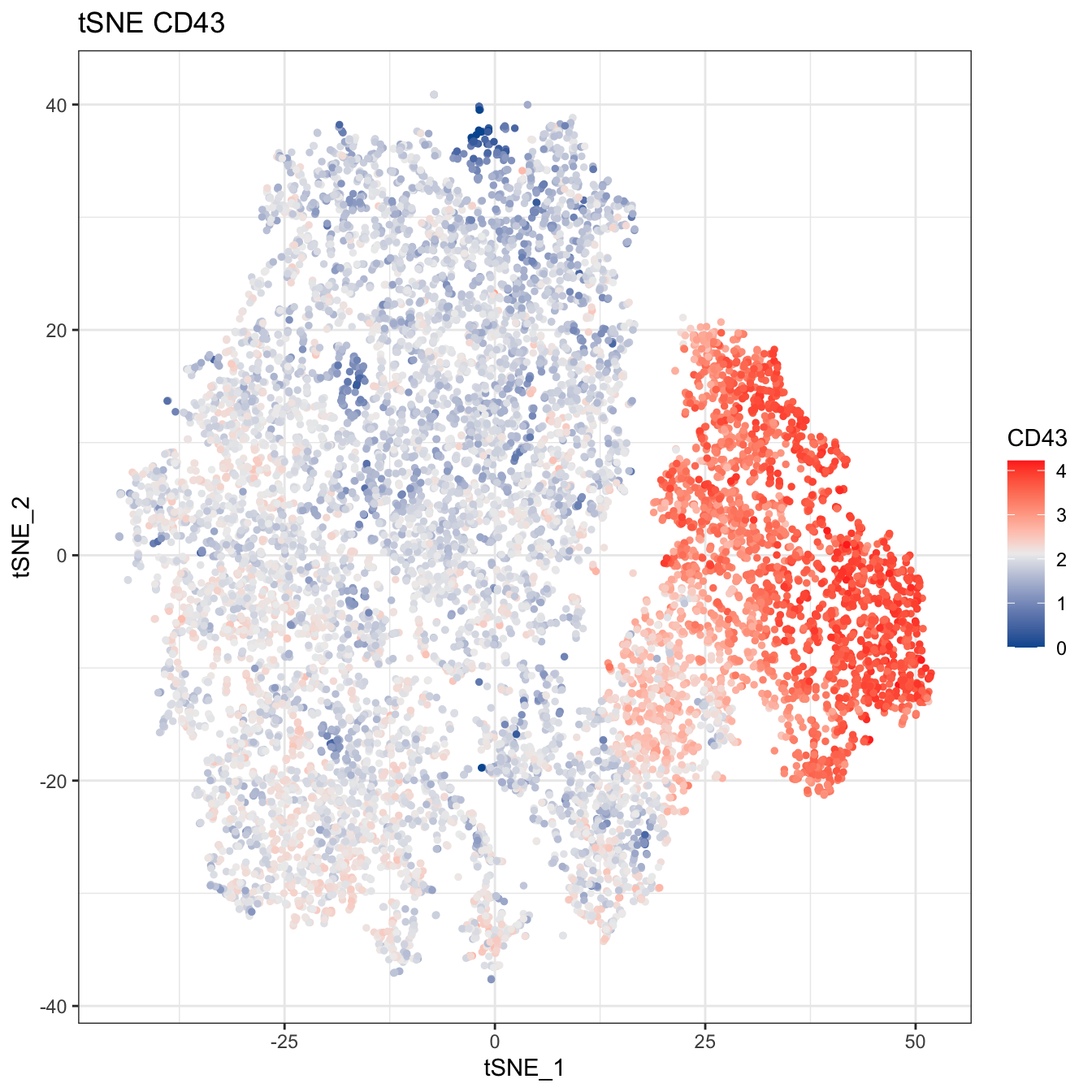

# Plot 2D UMAP. And cells are colored by CD43 markers expression
plot2D(cyt, item.use = c("UMAP_1", "UMAP_2"), color.by = "CD43", 
               main = "UMAP CD43", category = "numeric")  + 
 scale_colour_gradientn(colors = c("#00599F","#EEEEEE","#FF3222"))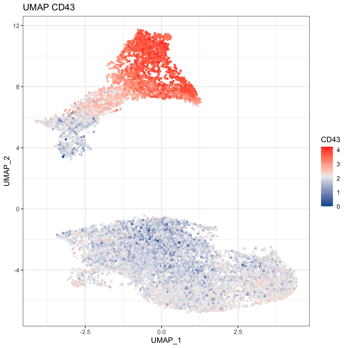

# Plot 2D UMAP. And cells are colored by stage
plot2D(cyt, item.use = c("UMAP_1", "UMAP_2"), color.by = "stage", 
       alpha = 1, main = "UMAP", category = "categorical") +
 scale_color_manual(values = c("#00599F","#009900","#FF9933",
                               "#FF99FF","#7A06A0","#FF3222"))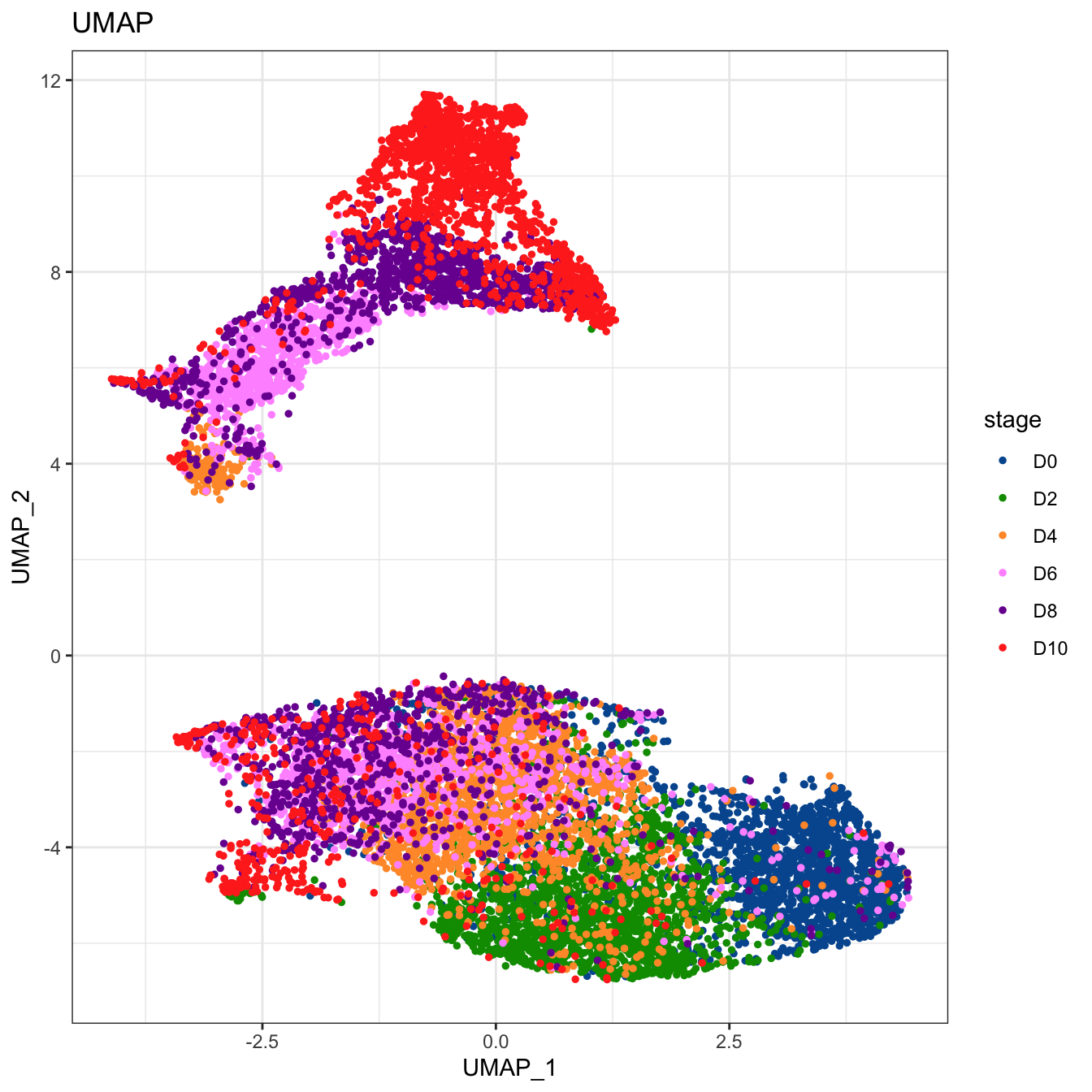

# Tree plot
plotTree(cyt, color.by = "CD49f", show.node.name = T, cex.size = 1) + 
  scale_colour_gradientn(colors = c("#00599F", "#EEEEEE", "#FF3222"))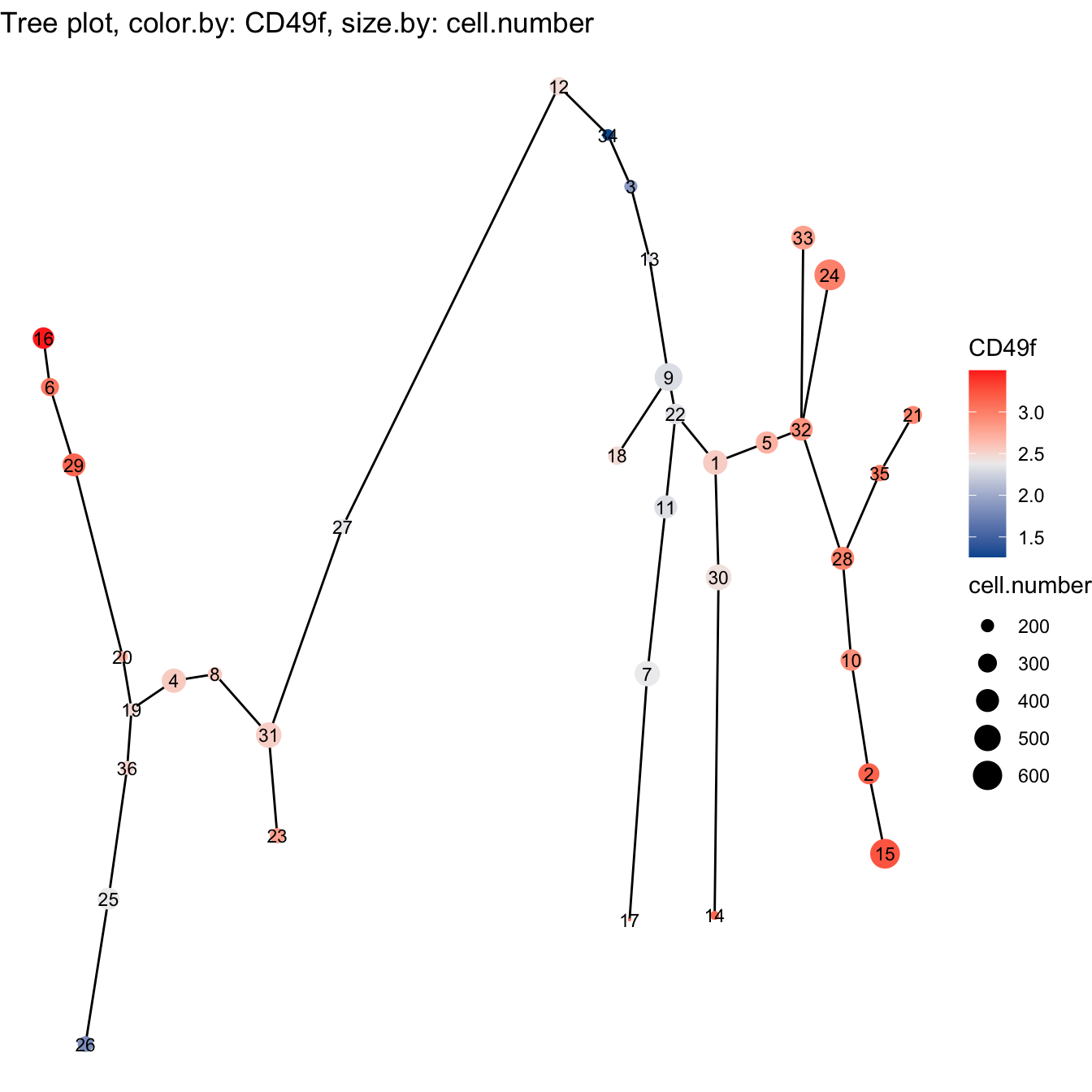

plotTree(cyt, color.by = "D0.percent", show.node.name = T, cex.size = 1) + 
  scale_colour_gradientn(colors = c("#00599F", "#EEEEEE", "#FF3222"))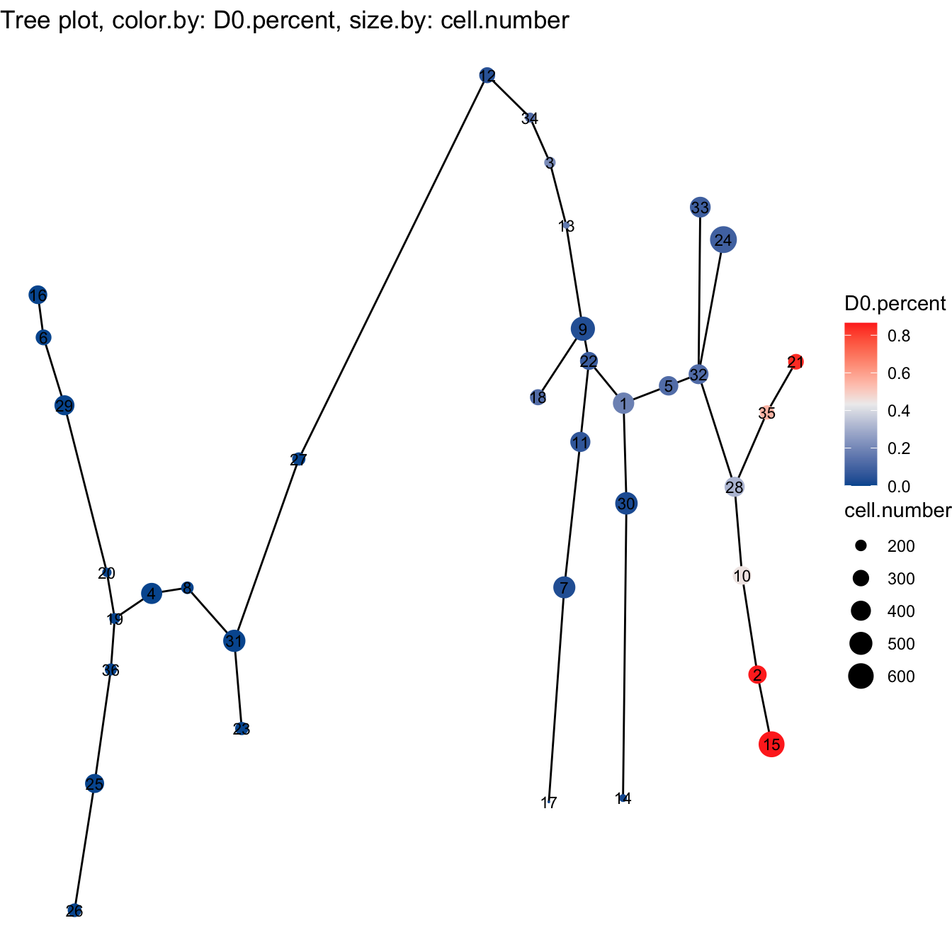

# plot clusters
plotCluster(cyt, item.use = c("PC_1", "PC_2"), category = "numeric",
            size = 10, color.by = "CD45RA") + 
  scale_colour_gradientn(colors = c("#00599F", "#EEEEEE", "#FF3222"))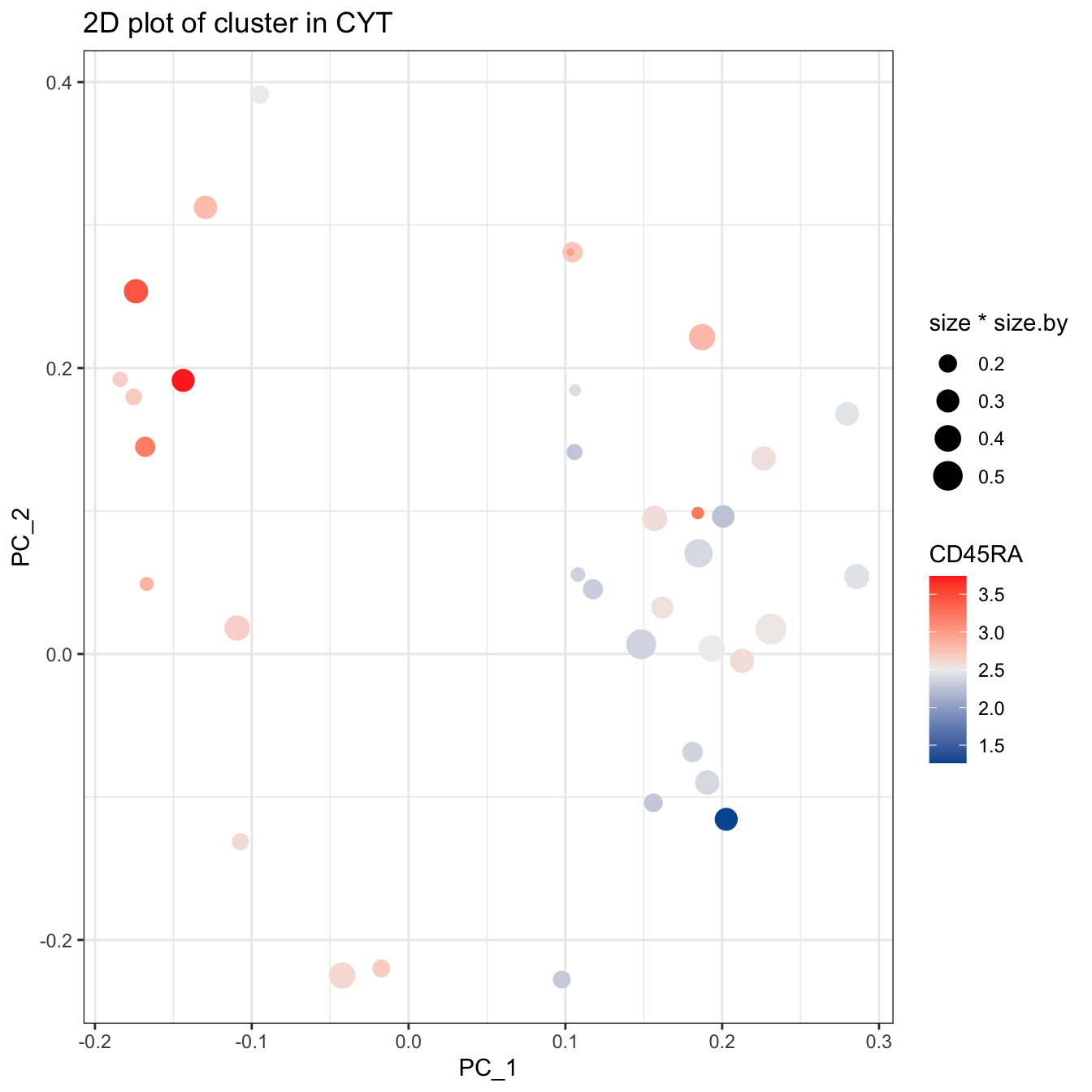

plotCluster(cyt, item.use = c("tSNE_1", "tSNE_2"), category = "numeric",
            size = 100, color.by = "CD45RA") + 
  scale_colour_gradientn(colors = c("#00599F", "#EEEEEE", "#FF3222"))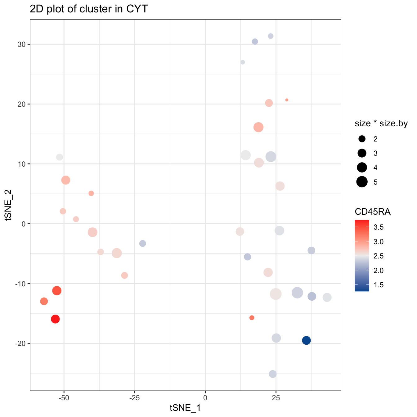

# plot pie tree
plotPieTree(cyt, cex.size = 3, size.by.cell.number = T) + 
 scale_fill_manual(values = c("#00599F","#009900","#FF9933",
                              "#FF99FF","#7A06A0","#FF3222"))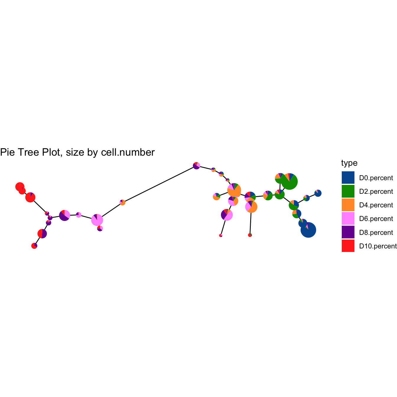

plotPieTree(cyt, cex.size = 5, size.by.cell.number = T, as.tree = T, root.id = 15) + 
 scale_fill_manual(values = c("#00599F","#009900","#FF9933",
                              "#FF99FF","#7A06A0","#FF3222"))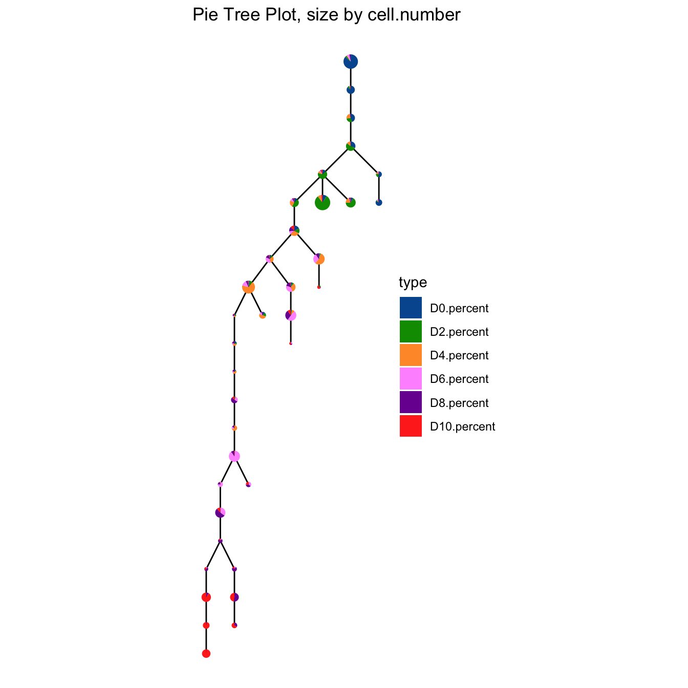

# plot pie cluster
plotPieCluster(cyt, item.use = c("tSNE_1", "tSNE_2"), cex.size = 50) + 
 scale_fill_manual(values = c("#00599F","#009900","#FF9933",
                              "#FF99FF","#7A06A0","#FF3222"))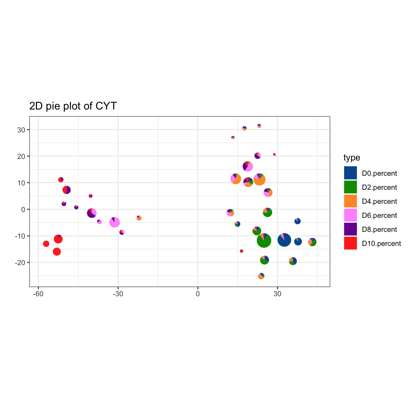

plotPieCluster(cyt, item.use = c("PC_1", "PC_2"), cex.size = 0.5) + 
 scale_fill_manual(values = c("#00599F","#009900","#FF9933",
                              "#FF99FF","#7A06A0","#FF3222"))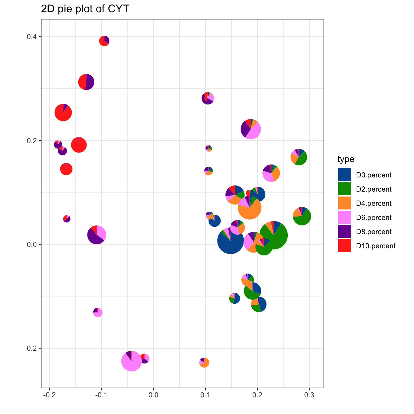

plotPieCluster(cyt, item.use = c("UMAP_1", "UMAP_2"), cex.size = 5) + 
 scale_fill_manual(values = c("#00599F","#009900","#FF9933",
                              "#FF99FF","#7A06A0","#FF3222"))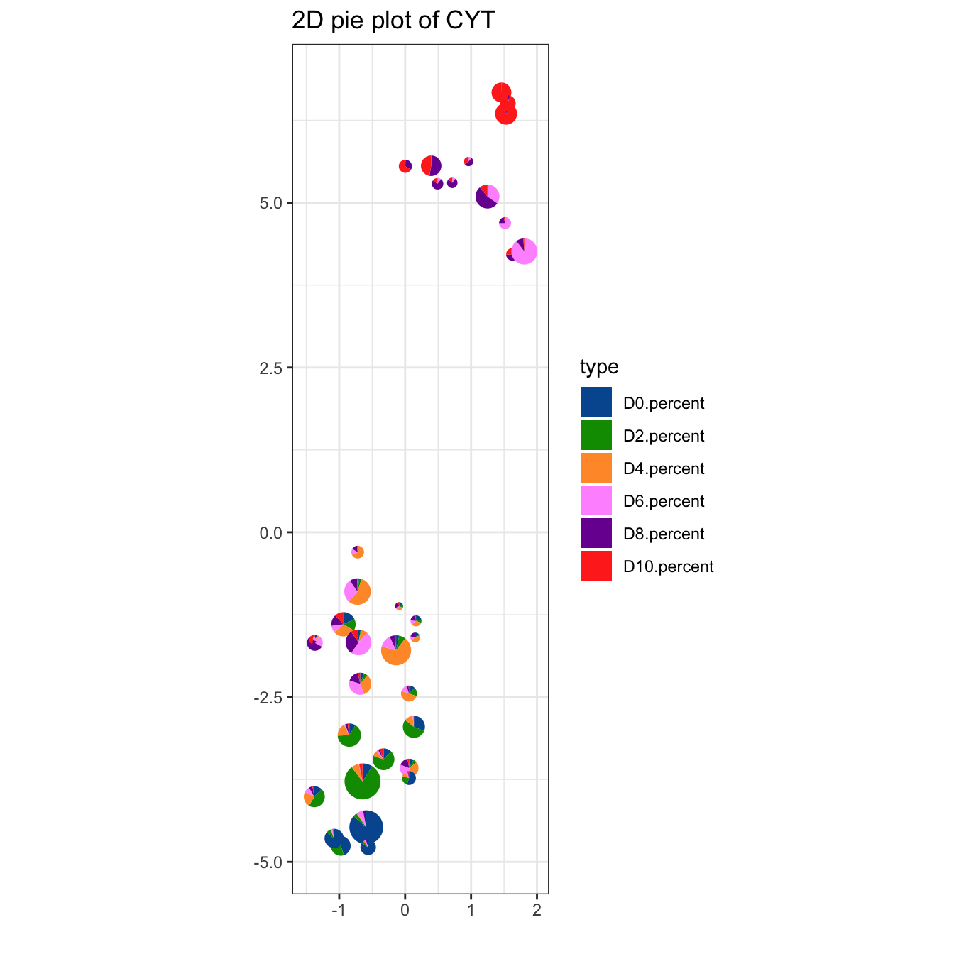

# plot cluster
plotCluster(cyt, item.use = c("tSNE_1", "tSNE_2"), size = 10, show.cluser.id = T)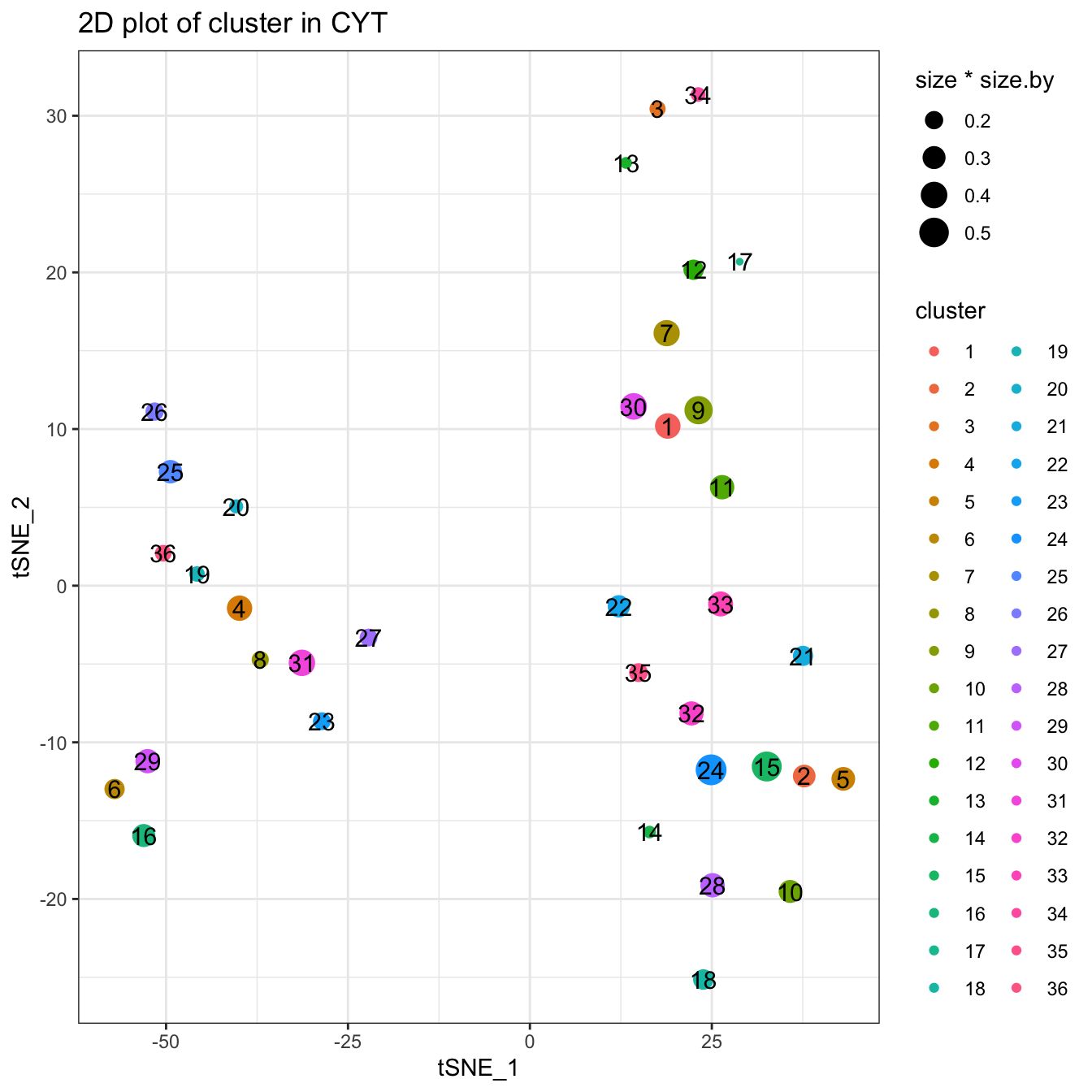

plotCluster(cyt, item.use = c("tSNE_1", "tSNE_2"), color.by = "CD43", 
            size = 10, show.cluser.id = T, category = "numeric") + 
 scale_colour_gradientn(colors = c("#00599F", "#EEEEEE", "#FF3222"))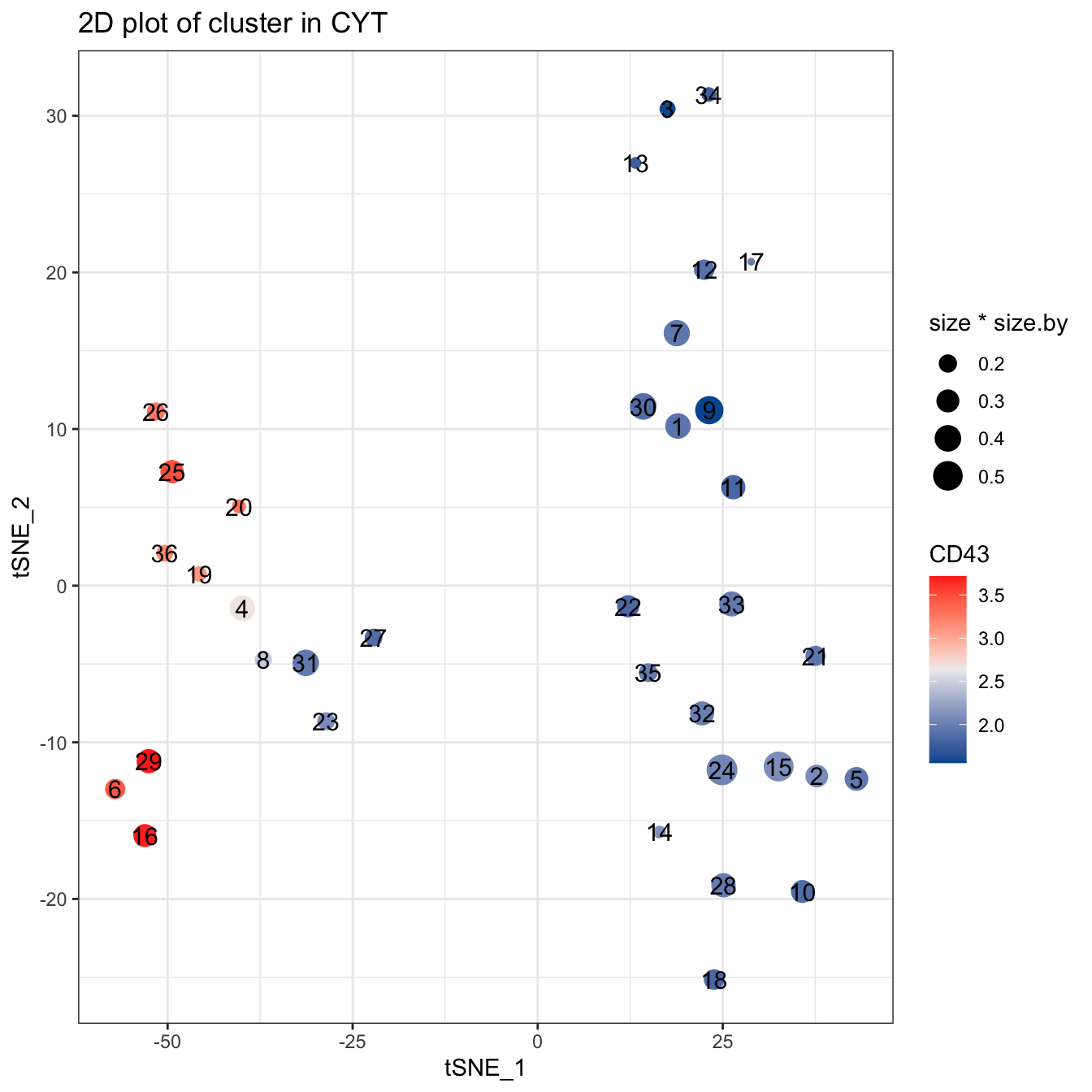

5.3 Step 3. Pseudotime

###########################################
# Pseudotime
###########################################

cyt <- defRootCells(cyt, root.cells = c(15))

cyt <- runPseudotime(cyt, verbose = T, dim.type = "raw")

## 2020-11-08 20:06:17 Calculating Pseudotime.

## 2020-11-08 20:06:17 The log data will be used to calculate pseudotime

## 2020-11-08 20:06:36 Calculating Pseudotime completed.

# tSNE plot colored by pseudotime
plot2D(cyt, item.use = c("tSNE_1", "tSNE_2"), category = "numeric",
            size = 1, color.by = "pseudotime") + 
 scale_colour_gradientn(colors = c("#F4D31D", "#FF3222","#7A06A0"))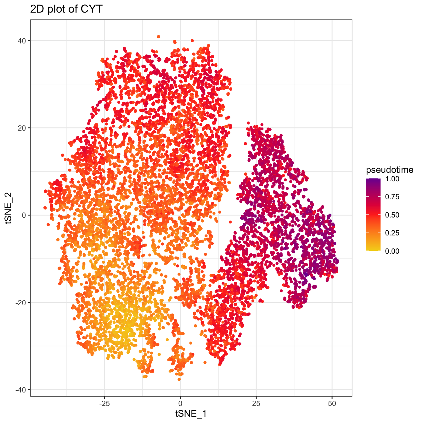

# UMAP plot colored by pseudotime
plot2D(cyt, item.use = c("UMAP_1", "UMAP_2"), category = "numeric",
            size = 1, color.by = "pseudotime") + 
 scale_colour_gradientn(colors = c("#F4D31D", "#FF3222","#7A06A0"))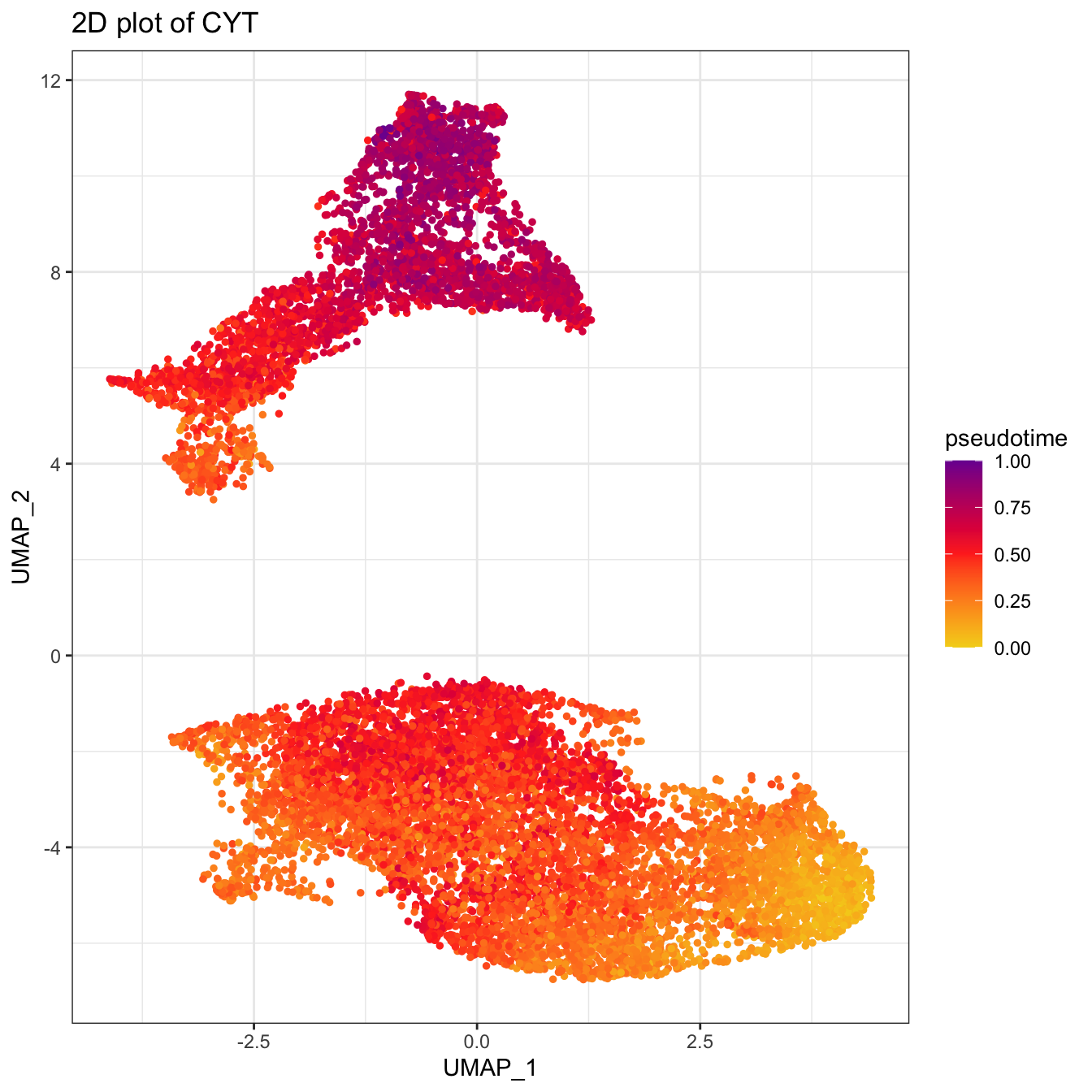

# Tree plot
plotTree(cyt, color.by = "pseudotime", cex.size = 1.5) + 
 scale_colour_gradientn(colors = c("#F4D31D", "#FF3222","#7A06A0"))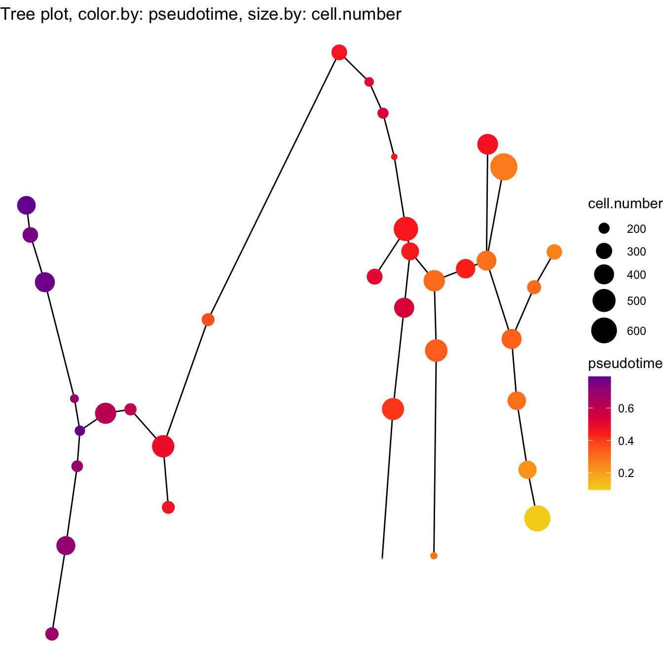

# denisty plot by different stage
plotPseudotimeDensity(cyt, adjust = 1) + 
 scale_color_manual(values = c("#00599F","#009900","#FF9933",
                               "#FF99FF","#7A06A0","#FF3222"))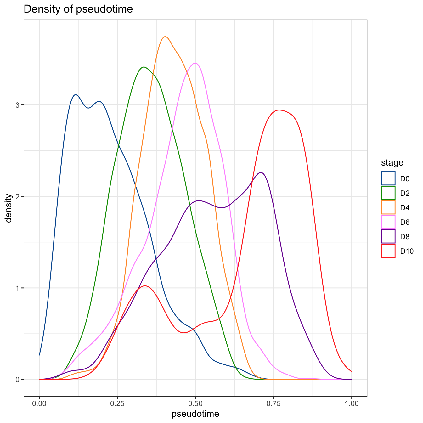

# trajectory value
plotPseudotimeTraj(cyt, var.cols = T) + 
 scale_colour_gradientn(colors = c("#F4D31D", "#FF3222","#7A06A0"))

## `geom_smooth()` using formula 'y ~ x'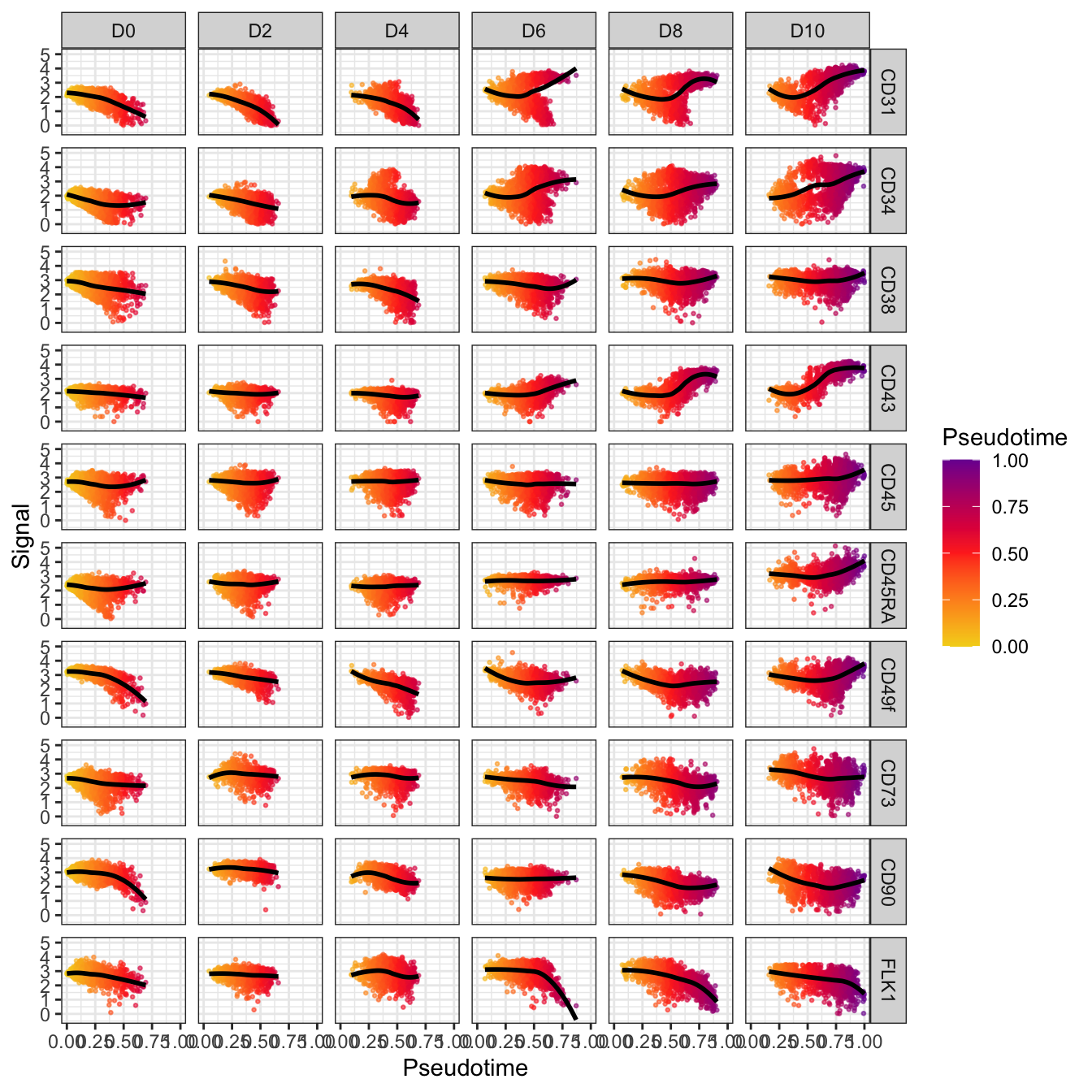

plotPseudotimeTraj(cyt, cutoff = 0.05, var.cols = T) + 
 scale_colour_gradientn(colors = c("#F4D31D", "#FF3222","#7A06A0"))

## `geom_smooth()` using formula 'y ~ x'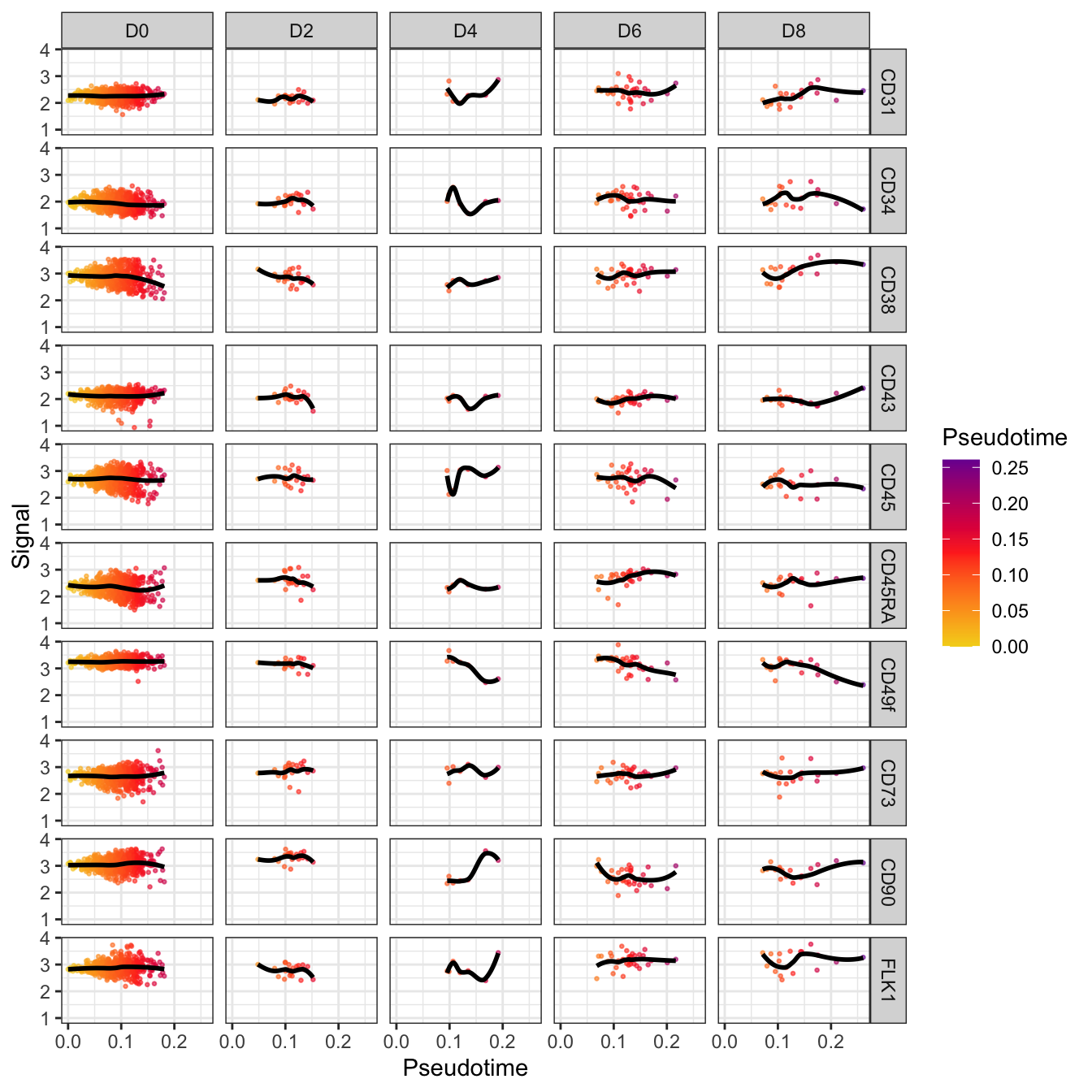

plotHeatmap(cyt, downsize = 1000, cluster_rows = T, clustering_method = "ward.D",
            color = colorRampPalette(c("#00599F","#EEEEEE","#FF3222"))(100))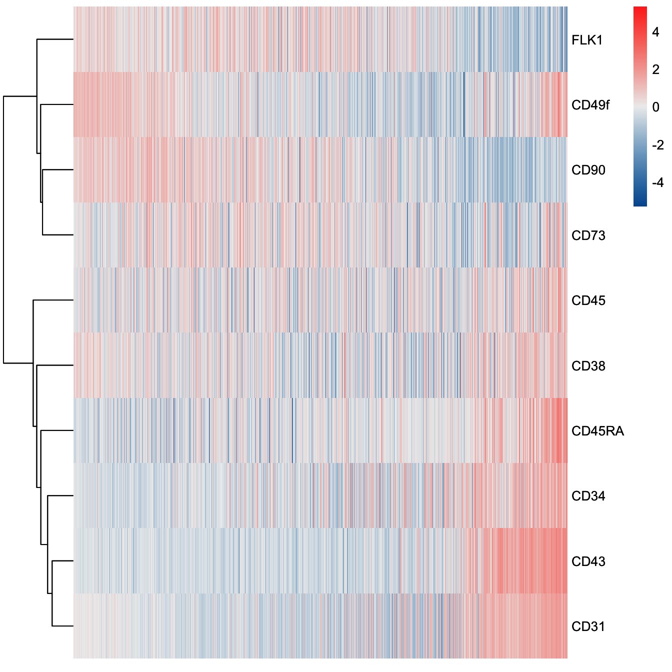

5.4 Step 4. Subset CYT

###########################################
# Subset CYT
###########################################

cell.inter <- fetchCell(cyt, cluster.id = c(26,25,36,19,4,8,31,20,29,6,16))
cell.inter <- cell.inter[grep("D6|D8|D10", cell.inter)]
sub.cyt <- subsetCYT(cyt, cells = cell.inter)

set.seed(1)
sub.cyt <- runCluster(sub.cyt, cluster.method = "som", xdim = 4, ydim = 4)

# Do not perform downsampling
set.seed(1)
sub.cyt <- processingCluster(sub.cyt, perplexity = 2, downsampling.size = 1)

# run Diffusion map
set.seed(1)
sub.cyt <- runDiffusionMap(sub.cyt)

sub.cyt <- defRootCells(sub.cyt, root.cells = c(13))

sub.cyt <- runPseudotime(sub.cyt, dim.type = "raw", dim.use = 1:2)

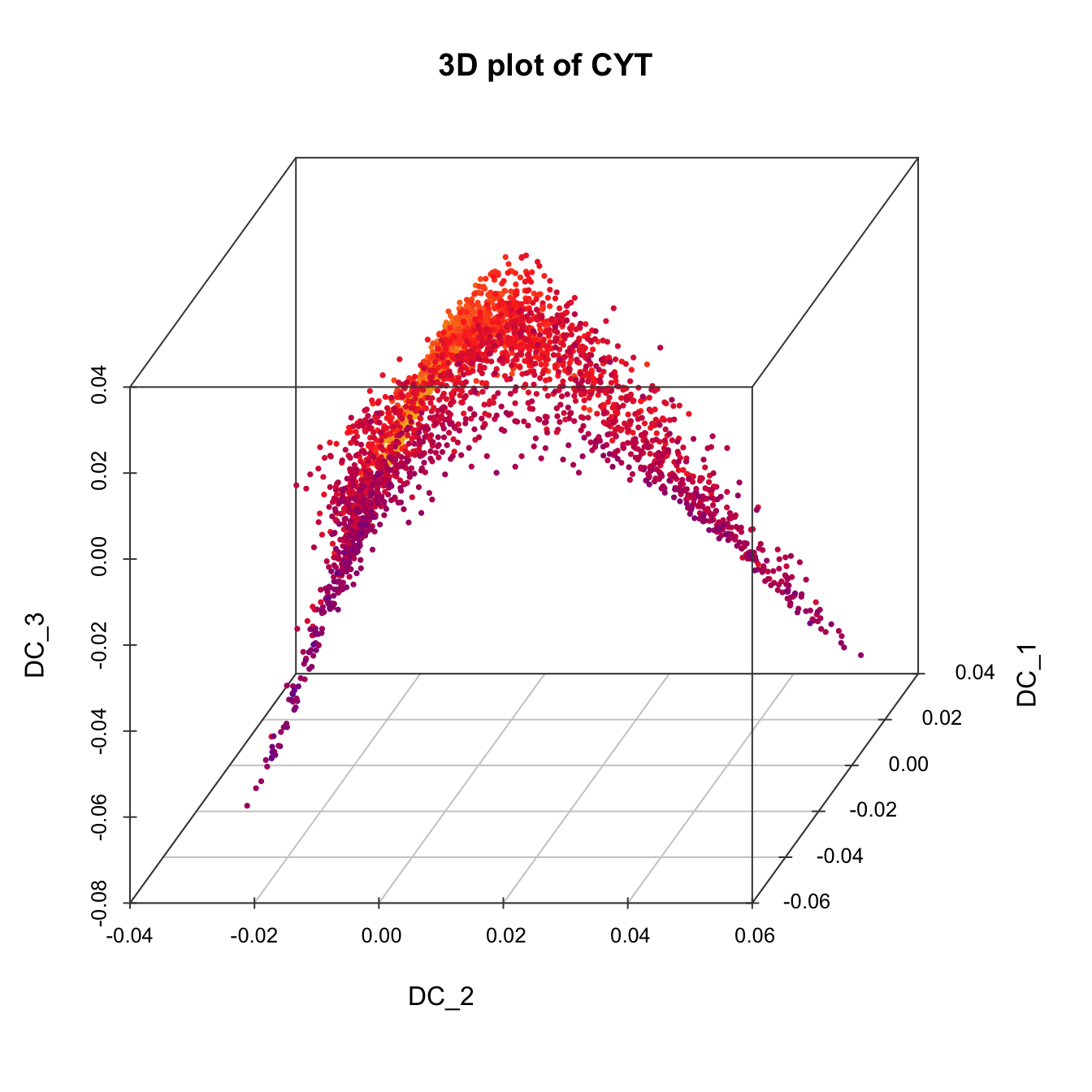
# 3D plot for CYT
plot3D(sub.cyt, item.use = c("DC_2","DC_1","DC_3"), color.by = "stage", 
       size = 0.5, angle = 60, color.theme = c("#FF99FF","#7A06A0","#FF3222"))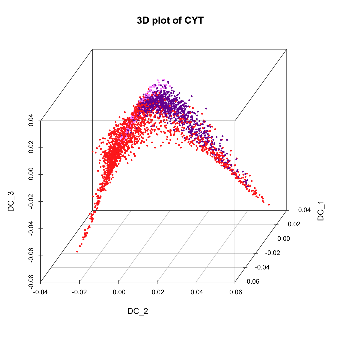

plot3D(sub.cyt, item.use = c("DC_2","DC_1","DC_3"), 
       size = 0.5, color.by = "CD49f", angle = 60,  category = "numeric",
       color.theme = c("#00599F","#00599F","#EEEEEE","#FF3222","#FF3222"))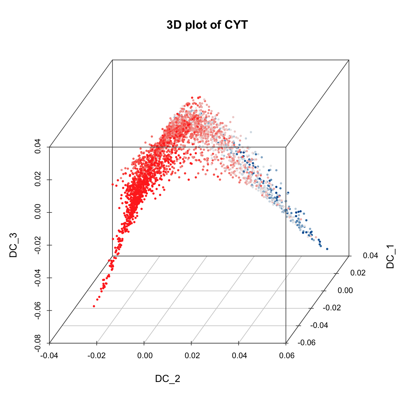

plot3D(sub.cyt, item.use = c("DC_2","DC_1","DC_3"), 
       size = 0.5, color.by = "CD43", angle = 60, category = "numeric",
       color.theme = c("#00599F","#00599F","#EEEEEE","#FF3222","#FF3222"))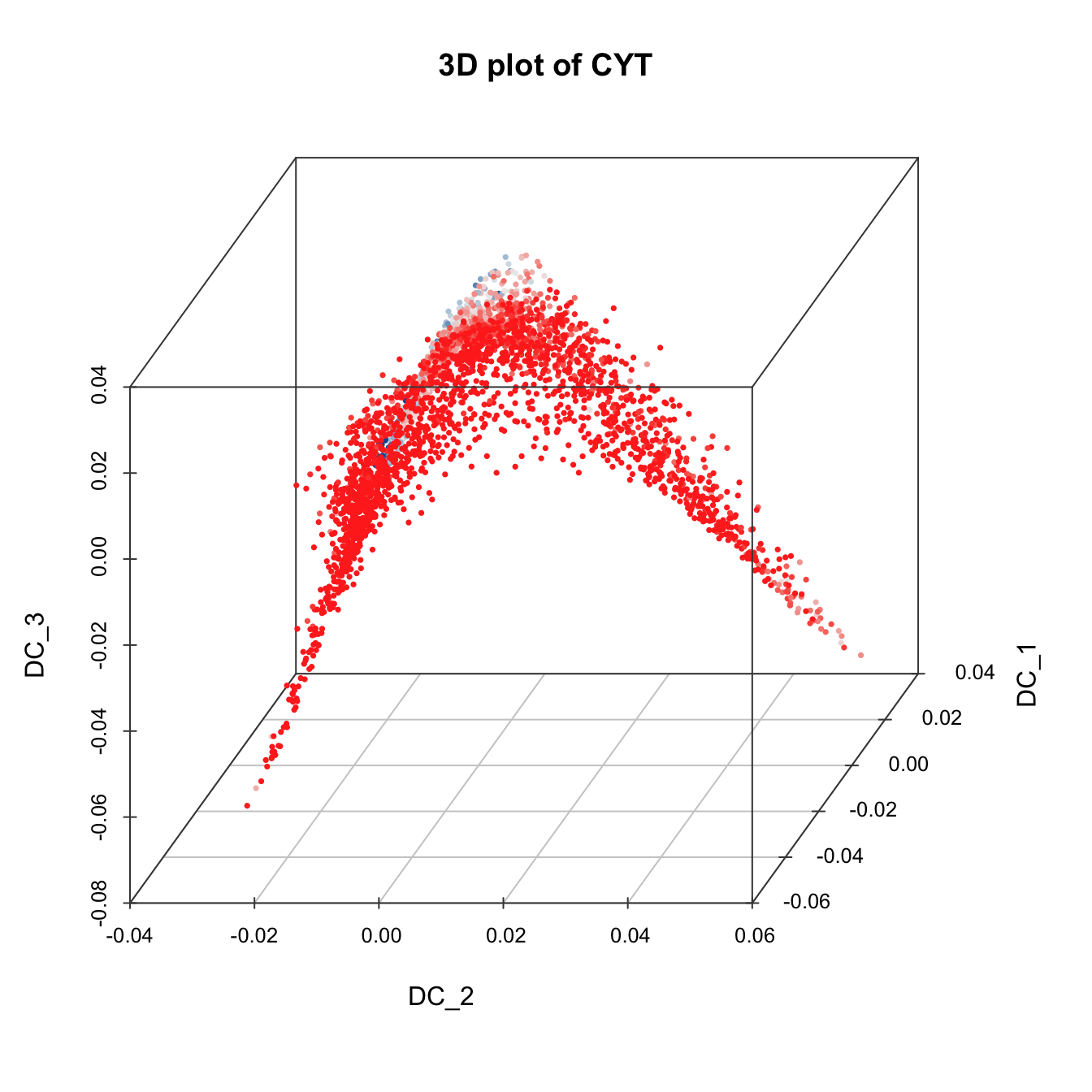

plot3D(sub.cyt, item.use = c("DC_2","DC_1","DC_3"), 
       size = 0.5, color.by = "pseudotime", angle = 60,  category = "numeric",
       color.theme = c("#F4D31D", "#FF3222","#7A06A0"))