Chapter 2 Quick Start

In this chapter, we will describe the four main functionalities of CytoTree and present the quick-start code template of CytoTree workflow. The data in this chapter are included in the CytoTree package. And through this chapter, you will learn:

1. The workflow of CytoTree.
1. How to build a CYT object.
1. A quick-start code template of CytoTree workflow.
1. A brief code template for visualization of CYT object.

And for the detailed version and advanced application of CytoTree, please read Chapter 3 and Chapter 4.

2.1 Overview of Workflow

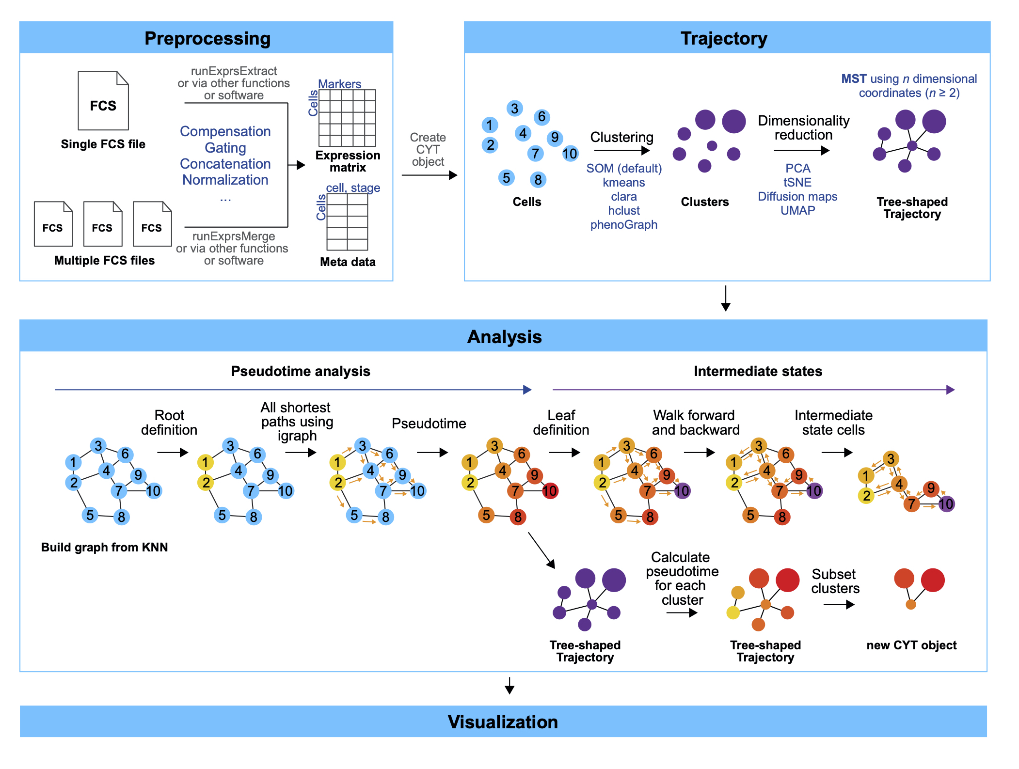
The CytoTree package is developed to complete the majority of standard analysis and visualization workflow for FCS data. In CytoTree workflow, an S4 object in R is built to implement the statistical and computational approach, and all computational functionalities are integrated into one single channel which only requires a specified input data format. Computational functionalities of CytoTree can be divided into four main parts (Fig. 2.1): preprocessing, trajectory, analysis and visualization.

Preprocessing. Data import, compensation, quality control, filtration, normalization and merge cells from different samples can be implemented in the preprocessing part. After preprocessing, a matrix that contains clean cytometric signaling data is required to build a CYT object. There are other optional data recommended to build the CYT object, including a data frame containing meta-information of the experiment and a vector contains all markers enrolled in the computational process.
Trajectory. Cells built in the CYT object are classified into different clusters based on the expression level of input markers. You can choose different clustering methods by inputting different parameters. After clustering, cells are downsampled in a cluster-dependent fashion to reduce the total cell size and avoid small cluster deletion. Dimensionality reduction for both cells and clusters are also implemented in the clustering procedure. After dimensionality reduction, we use Minimus Spanning Tree (MST) to construct cell trajectory.
Analysis. This part is designed for time course FCS data. Before running pseudotime, root cells must be defined first based on users’ prior knowledge. Root cells in CytoTree workflow are the initial cells of the trajectory tree. So it can be set using one vertex node of the tree or a cluster of cells with specific antibodies combination. Intermediate state evaluation is also involved in the pseudotime part. Leaf cells are defined by the end node of the trajectory or the end stage of the experiment. Intermediate state cells are cells with higher betweenness in the graph built on cell-cell connection, which plays an important role between the connection of root cells and leaf cells.
Visualization. The visualization part can provide clear and concise visualization of FCS data in an effective and easy-to-comprehend manner. CytoTree package offers various plotting functions to generate customizable and publication-quality plots. A two-dimensional or three-dimensional plot can fit most requirements from dimensionality reduction results. And tree-based plot can visualize cell trajectory as a force-directed layout tree. Other special plots such as heatmap and violin plot are also provided in CytoTree.

Figure 2.1 Workflow of CytoTree

2.2 Installation

2.2.1 GitHub

This requires the devtools package to be pre-installed first.

# If not already installed
install.packages("devtools") 
devtools::install_github("JhuangLab/CytoTree")

library(CytoTree)

The link of CytoTree on GitHub can be visited at https://github.com/JhuangLab/CytoTree.

2.2.2 Bioconductor

This requires the BiocManager package to be pre-installed first, and make sure the version of Bioc is 3.12.

To install this package, start R (version “4.0”) and enter:

if (!requireNamespace("BiocManager", quietly = TRUE))
    install.packages("BiocManager")

BiocManager::install("CytoTree")

The link of CytoTree on Bioconductor can be visited at https://bioconductor.org/packages/CytoTree/.

2.3 Quick-start code

To run CytoTree, the first step is to build a CYT object. Here are the main functions in CytoTree. This figure describes the available functionalities: preprocessing, trajectory, analysis, visualization, and set operations. A short description (black font) and the corresponding function (blue font) are provided for each function. The CytoTree workflow begins with the reading of the FCS data. Compensation, filtration, concatenation, and normalization are included in the preprocessing part. A clean matrix after preprocessing is required to build a CYT object, and the analysis workflows of all other functionalities are all based on the CYT object. The trajectory module contains functions used to perform clustering and dimensionality reduction for cells. The analysis module is based on calculation results from the trajectory part. The visualization part includes functions to generate publication-quality plots from the CYT object. The set operations part includes a function for subsetting a CYT object based on user-defined cells or fetching meta information for clusters and cells during the analysis.

# Loading packages
suppressMessages({
library(CytoTree)
})

# Read fcs files
fcs.path <- system.file("extdata", package = "CytoTree")
fcs.files <- list.files(fcs.path, pattern = '.FCS$', full = TRUE)

# Using runExprsMerge for multip FCS files
# Or using runExprsExtract for one single FCS file
fcs.data <- runExprsMerge(fcs.files, comp = FALSE, transformMethod = "none")

# Build the CYT object
cyt <- createCYT(raw.data = fcs.data, normalization.method = "log")

# See information
cyt

## CYT Information:
##  Input cell number: 600  cells 
##  Enroll marker number: 18  markers 
##  Cells after downsampling: 600  cells

################################################
##### Running CytoTree in one line code
################################################

# Run without dimensionality reduction steps
# Run CytoTree as pipeline and visualize as tree
cyt <- cyt %>% runCluster() %>% processingCluster() %>% buildTree()
plotTree(cyt)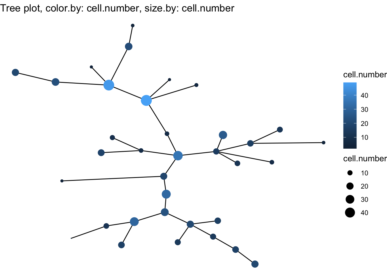

# Or you can run with dimensionality reduction steps
# Run CytoTree as pipeline and visualize as tree
cyt <- cyt %>% runCluster() %>% processingCluster() %>% 
  runFastPCA() %>% runTSNE() %>%  runDiffusionMap() %>% runUMAP() %>% 
  buildTree()
plot2D(cyt, item.use = c("UMAP_1", "UMAP_2"))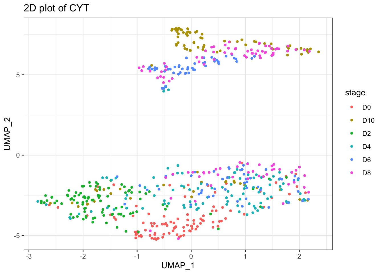

Here we provide the running template of trajectory inference using CYT object is as follows:

# Cluster cells by SOM algorithm
set.seed(1)
cyt <- runCluster(cyt)

# Processing Clusters
cyt <- processingCluster(cyt)

# This is an optional step
# run Principal Component Analysis (PCA)
cyt <- runFastPCA(cyt)

# This is an optional step
# run t-Distributed Stochastic Neighbor Embedding (tSNE)
cyt <- runTSNE(cyt)

# This is an optional step
# run Diffusion map
cyt <- runDiffusionMap(cyt)

# This is an optional step
# run Uniform Manifold Approximation and Projection (UMAP)
cyt <- runUMAP(cyt)

# build minimum spanning tree
cyt <- buildTree(cyt)

# DEGs of different branch
diff.list <- runDiff(cyt)

# define root cells
cyt <- defRootCells(cyt, root.cells = c(32,26))

# run pseudotime
cyt <- runPseudotime(cyt)

# define leaf cells
cyt <- defLeafCells(cyt, leaf.cells = c(30))

# run walk between root cells and leaf cells
cyt <- runWalk(cyt)

# Save object
if (FALSE) {
  saveRDS(cyt, file = "Path to you output directory")
}

2.4 Visualization

The running template of visualization is as follows:

# Plot 2D tSNE. And cells are colored by cluster id
plot2D(cyt, item.use = c("tSNE_1", "tSNE_2"), color.by = "cluster.id", 
       alpha = 1, main = "tSNE", category = "categorical", show.cluser.id = TRUE)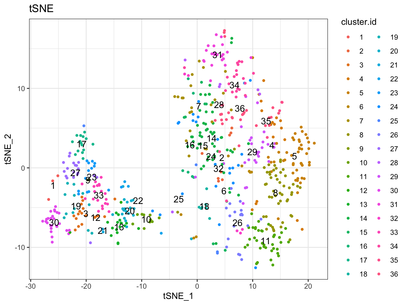

# Plot 2D UMAP. And cells are colored by cluster id
plot2D(cyt, item.use = c("UMAP_1", "UMAP_2"), color.by = "cluster.id", 
       alpha = 1, main = "UMAP", category = "categorical", show.cluser.id = TRUE)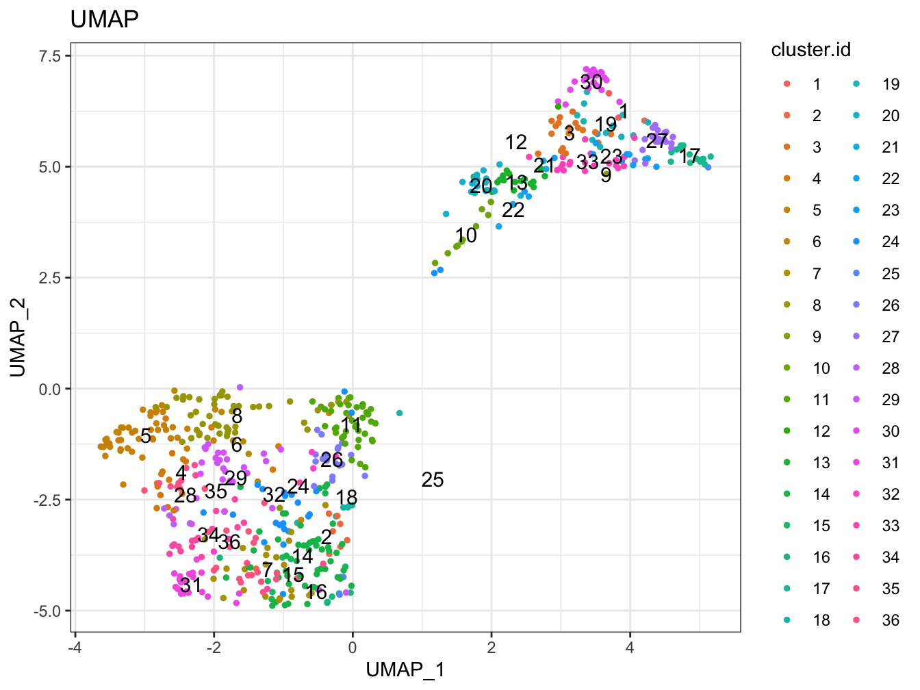

# Plot 2D tSNE. And cells are colored by cluster id
plot2D(cyt, item.use = c("tSNE_1", "tSNE_2"), color.by = "branch.id", 
       alpha = 1, main = "tSNE", category = "categorical", show.cluser.id = TRUE)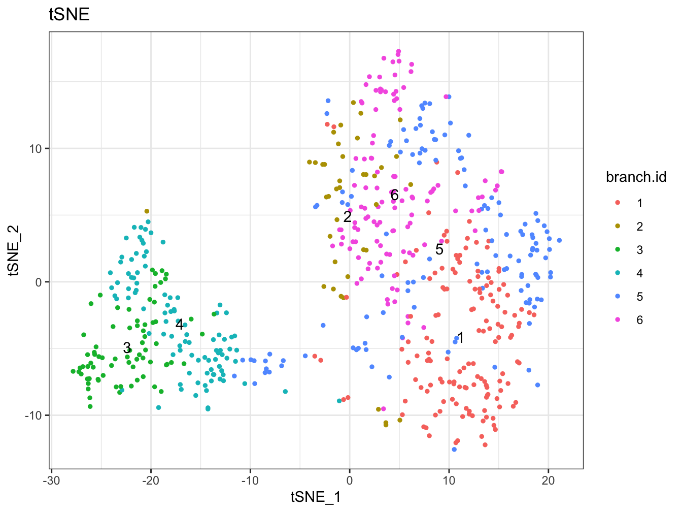

# Plot 2D UMAP. And cells are colored by cluster id
plot2D(cyt, item.use = c("UMAP_1", "UMAP_2"), color.by = "branch.id", 
       alpha = 1, main = "UMAP", category = "categorical", show.cluser.id = TRUE)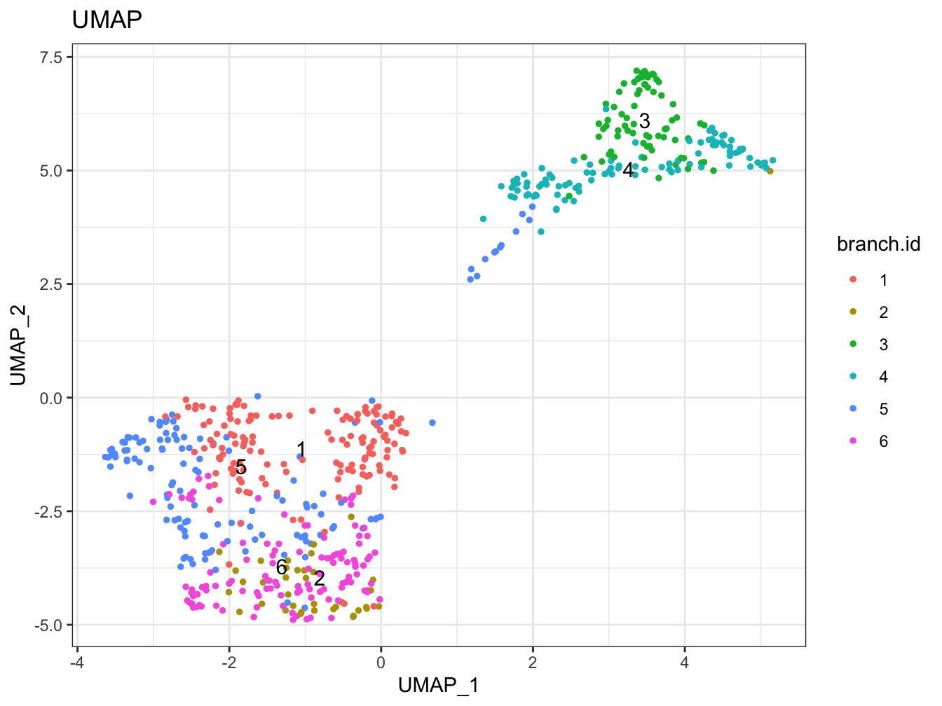

# Plot 2D tSNE. And cells are colored by stage
plot2D(cyt, item.use = c("tSNE_1", "tSNE_2"), color.by = "stage", 
       alpha = 1, main = "UMAP", category = "categorical")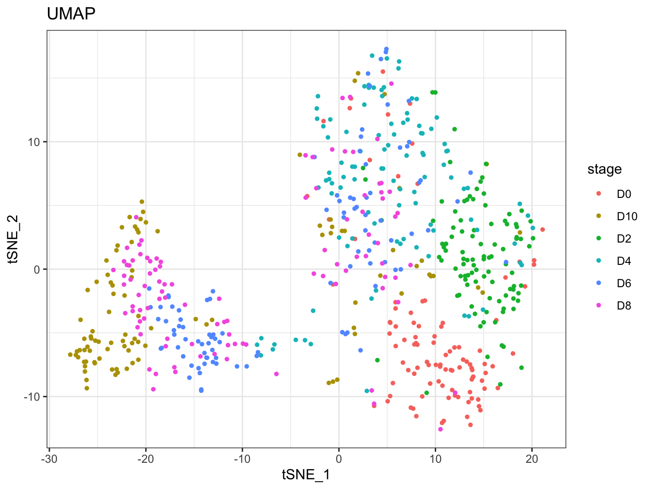

# Plot 2D UMAP. And cells are colored by stage
plot2D(cyt, item.use = c("UMAP_1", "UMAP_2"), color.by = "stage", 
       alpha = 1, main = "UMAP", category = "categorical")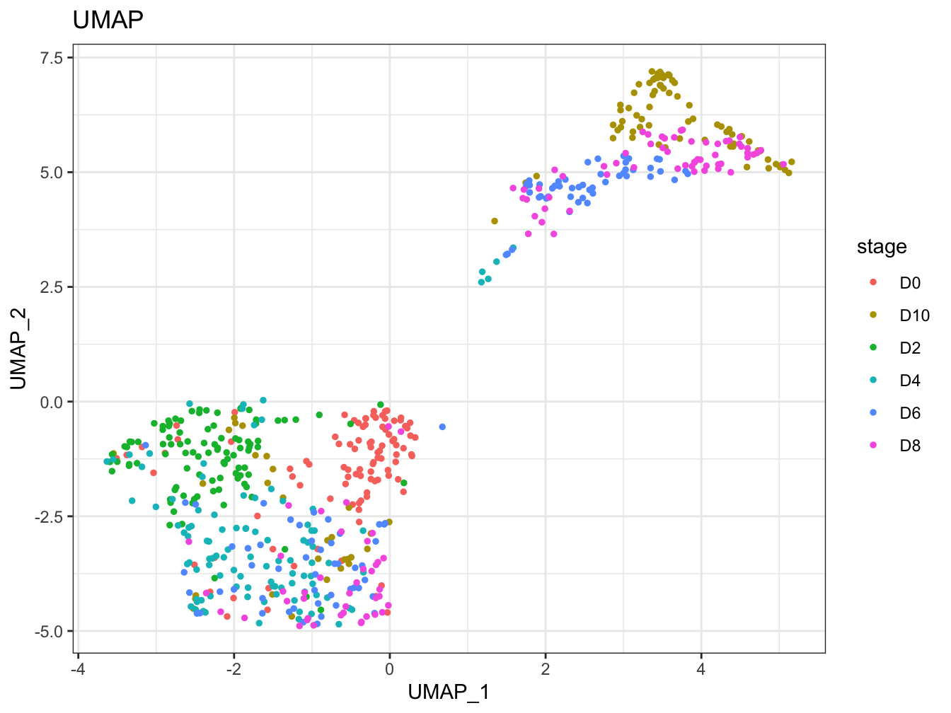

# Tree plot
plotTree(cyt, color.by = "D0.percent", show.node.name = TRUE, cex.size = 1)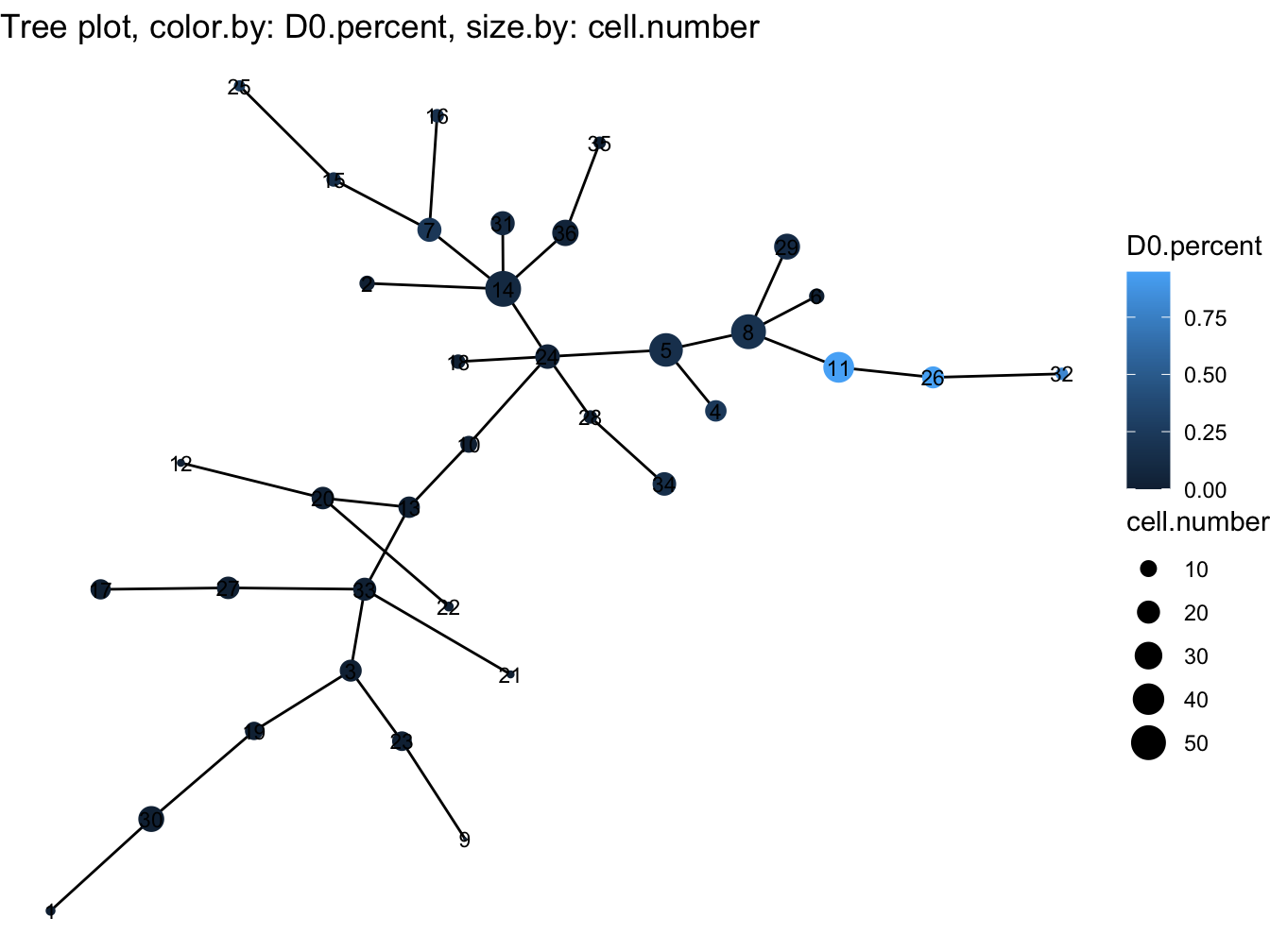

# Tree plot
plotTree(cyt, color.by = "FITC-A<CD43>", show.node.name = TRUE, cex.size = 1)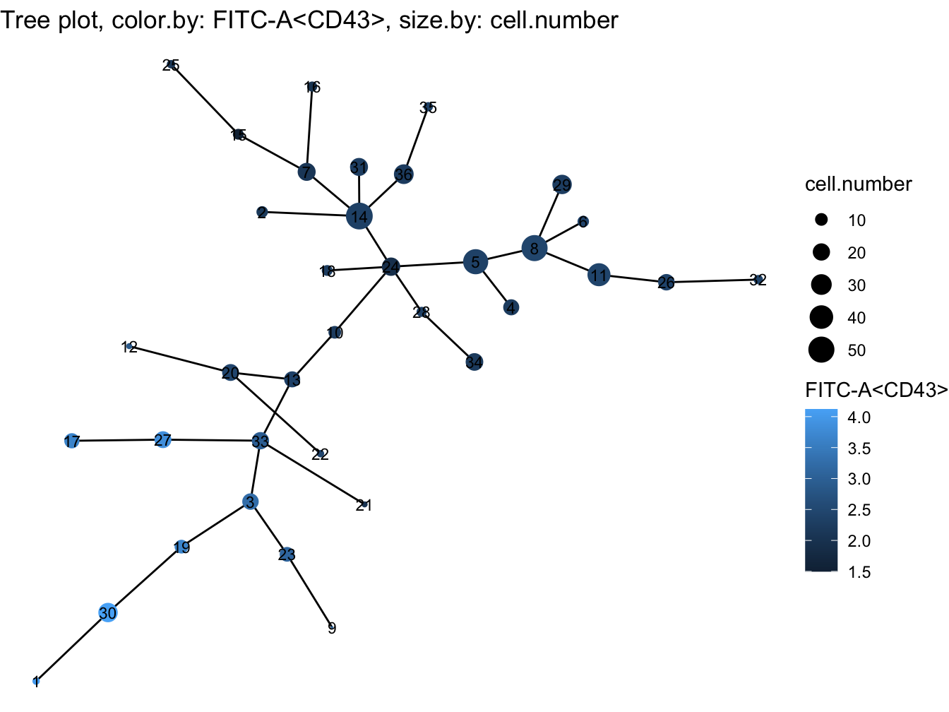

# plot clusters
plotCluster(cyt, item.use = c("tSNE_1", "tSNE_2"), category = "numeric",
            size = 100, color.by = "BV510-A<CD45RA>")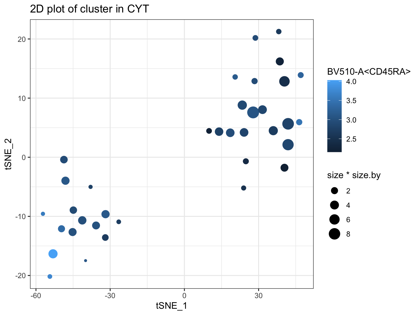

# plot pie tree
plotPieTree(cyt, cex.size = 3, size.by.cell.number = TRUE)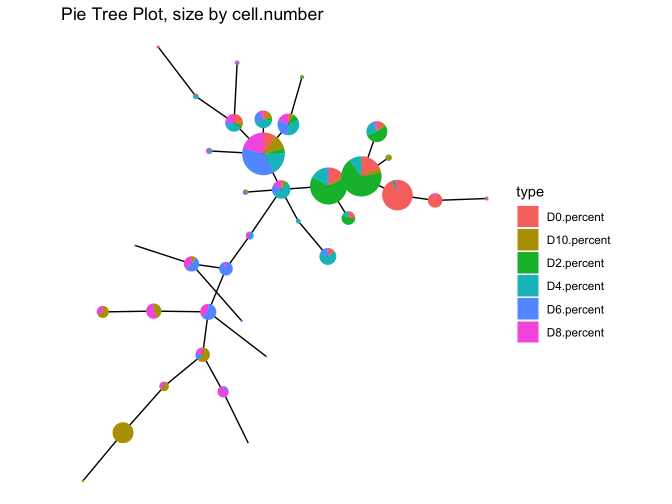

# plot pie cluster
plotPieCluster(cyt, item.use = c("tSNE_1", "tSNE_2"), cex.size = 40)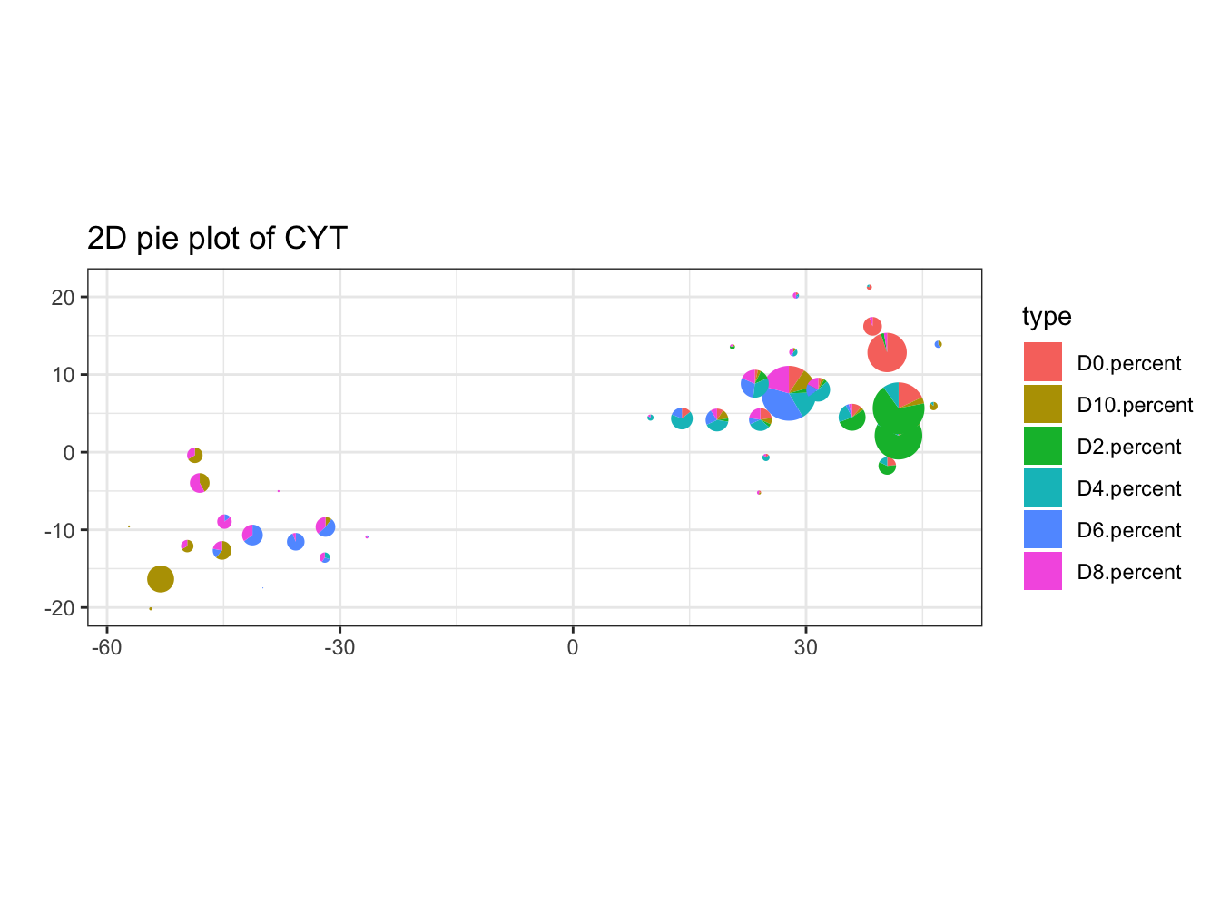

# plot heatmap of clusters
plotClusterHeatmap(cyt)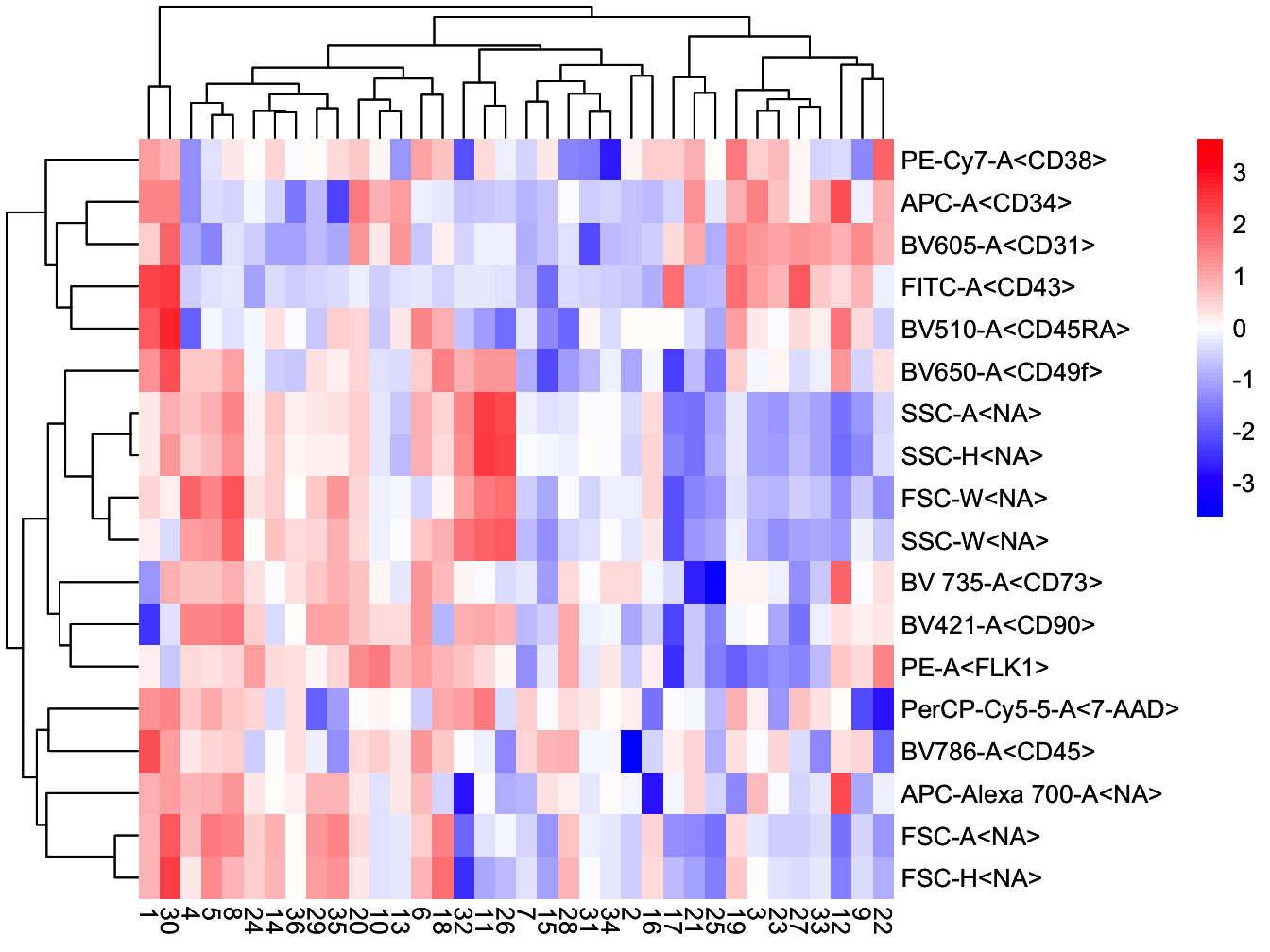

# plot heatmap of branches
plotBranchHeatmap(cyt)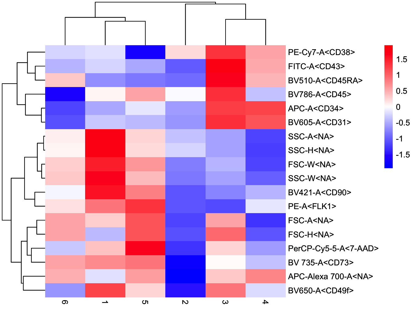

# Violin plot
plotViolin(cyt, color.by = "cluster.id", marker = "BV510-A<CD45RA>", text.angle = 90)

## Warning: `fun.y` is deprecated. Use `fun` instead.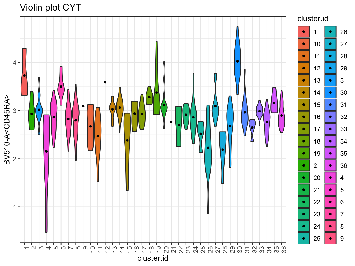

# Violin plot
plotViolin(cyt, color.by = "branch.id", marker = "BV510-A<CD45RA>", text.angle = 90)

## Warning: `fun.y` is deprecated. Use `fun` instead.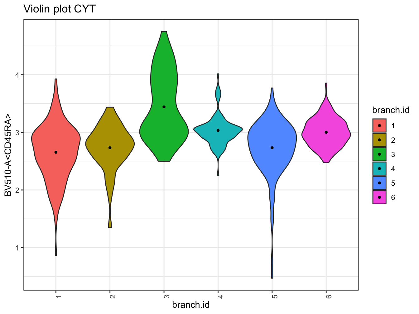

# UMAP plot colored by pseudotime
plot2D(cyt, item.use = c("UMAP_1", "UMAP_2"), category = "numeric",
            size = 1, color.by = "pseudotime")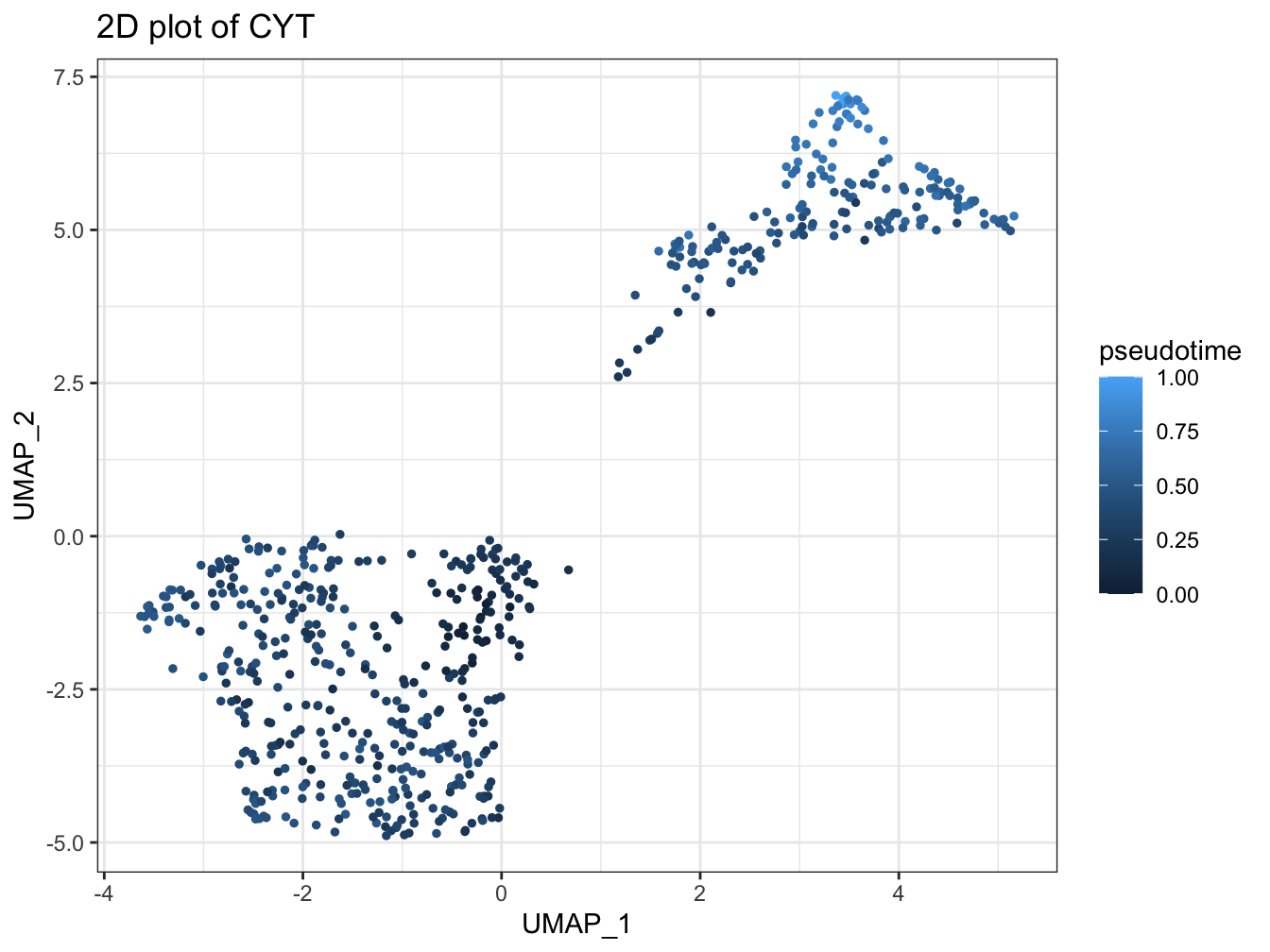

# tSNE plot colored by pseudotime
plot2D(cyt, item.use = c("tSNE_1", "tSNE_2"), category = "numeric",
            size = 1, color.by = "pseudotime")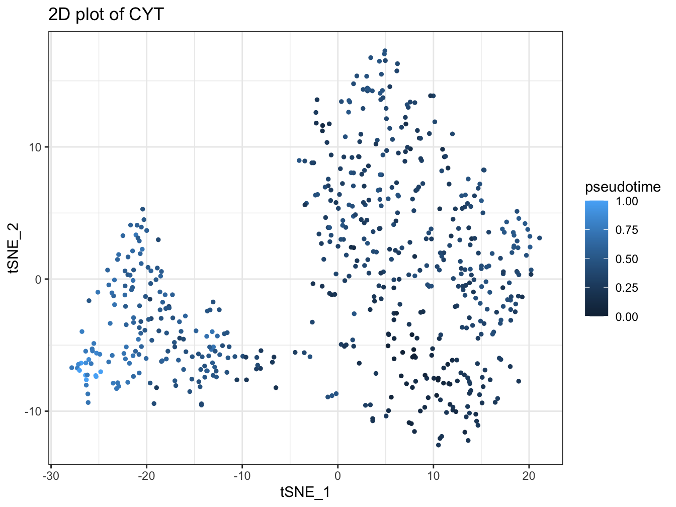

# denisty plot by different stage
plotPseudotimeDensity(cyt, adjust = 1)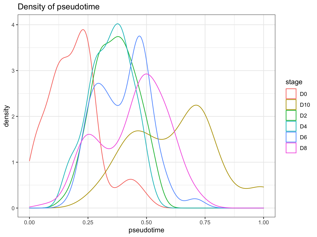

# Tree plot
plotTree(cyt, color.by = "pseudotime", cex.size = 1.5)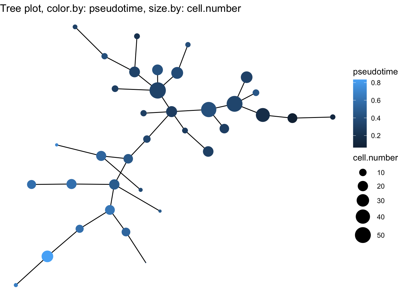

# Violin plot
plotViolin(cyt, color.by = "cluster.id", order.by = "pseudotime",
           marker = "BV650-A<CD49f>", text.angle = 90)

## Warning: `fun.y` is deprecated. Use `fun` instead.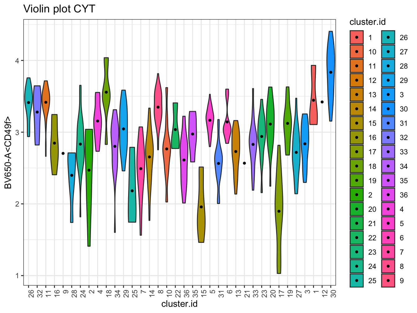

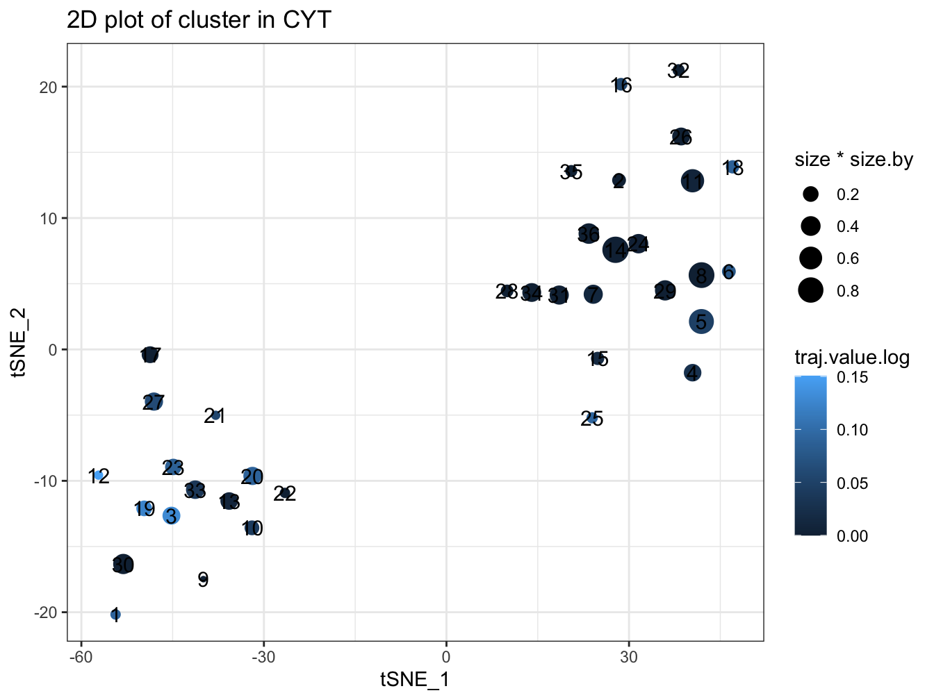
# trajectory value
plotPseudotimeTraj(cyt, var.cols = TRUE)

## `geom_smooth()` using formula 'y ~ x'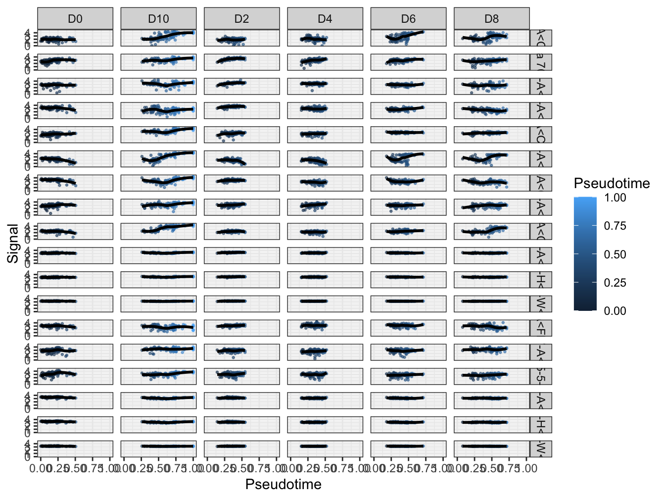

# Heatmap plot
plotHeatmap(cyt, downsize = 1000, cluster_rows = TRUE, clustering_method = "ward.D",
            color = colorRampPalette(c("#00599F","#EEEEEE","#FF3222"))(100))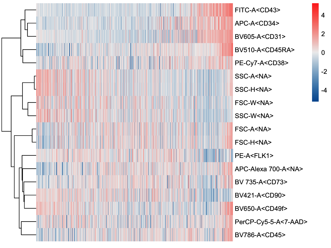

# plot cluster
plotCluster(cyt, item.use = c("tSNE_1", "tSNE_2"), color.by = "traj.value.log", 
            size = 10, show.cluser.id = TRUE, category = "numeric")